Explained: Deep learning methods for scRNA-seq clustering

DESC^[1] and scDCC^[2] are two popular deep learning-based methods for the clustering of single cell data (specifically, scRNA-seq count matrices). In the post I'll assume some familiarity with single cell expression data. Additionally, it is also helpful to have some background knowledge on autoencoders, though not completely necessary. I'll cover variational autoencoder (VAE) based methods such as scGen^[3] and scvis^[4]  in a future post. For now, I'll cover how DESC and scDCC implement a specialized clustering loss  function to generate more ideal cell embeddings.

Autoencoders

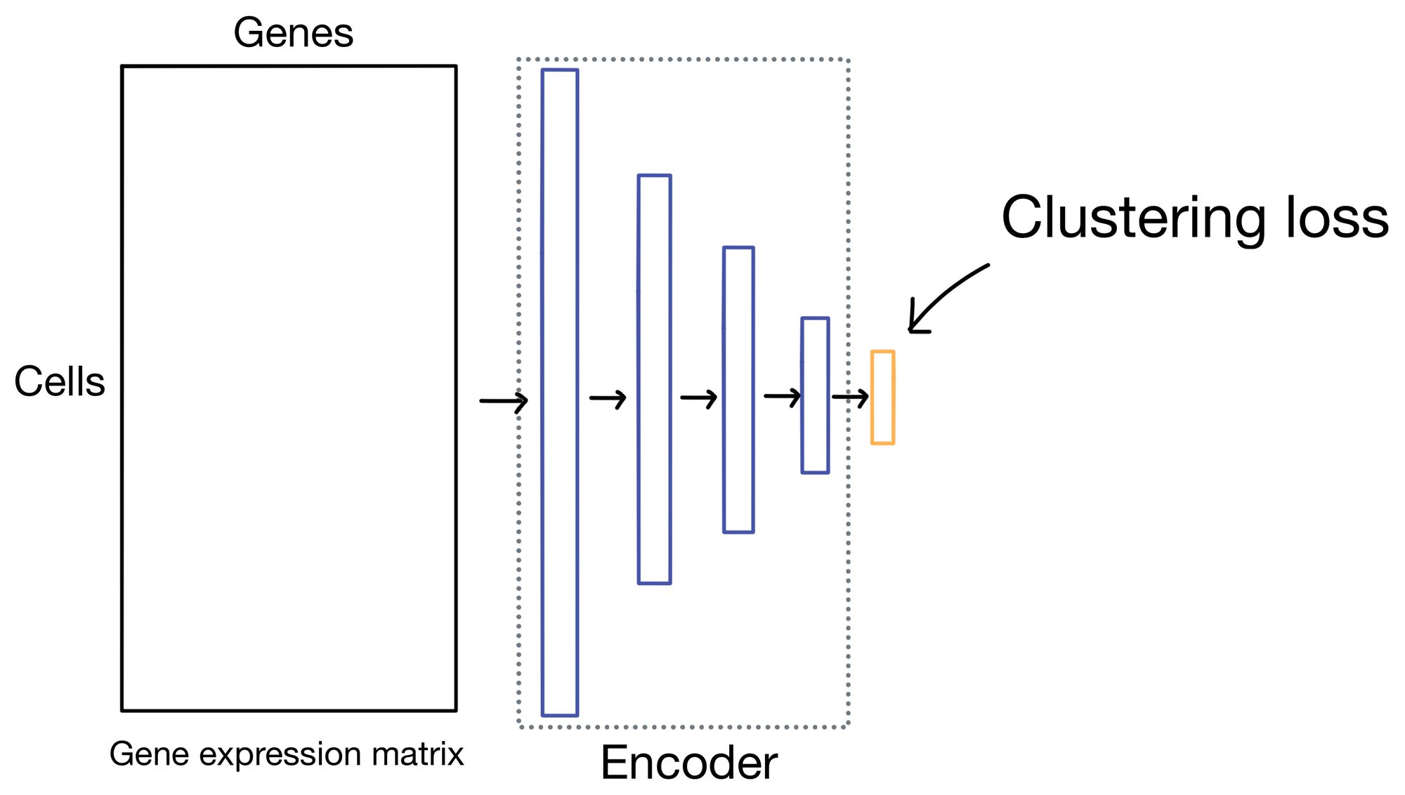
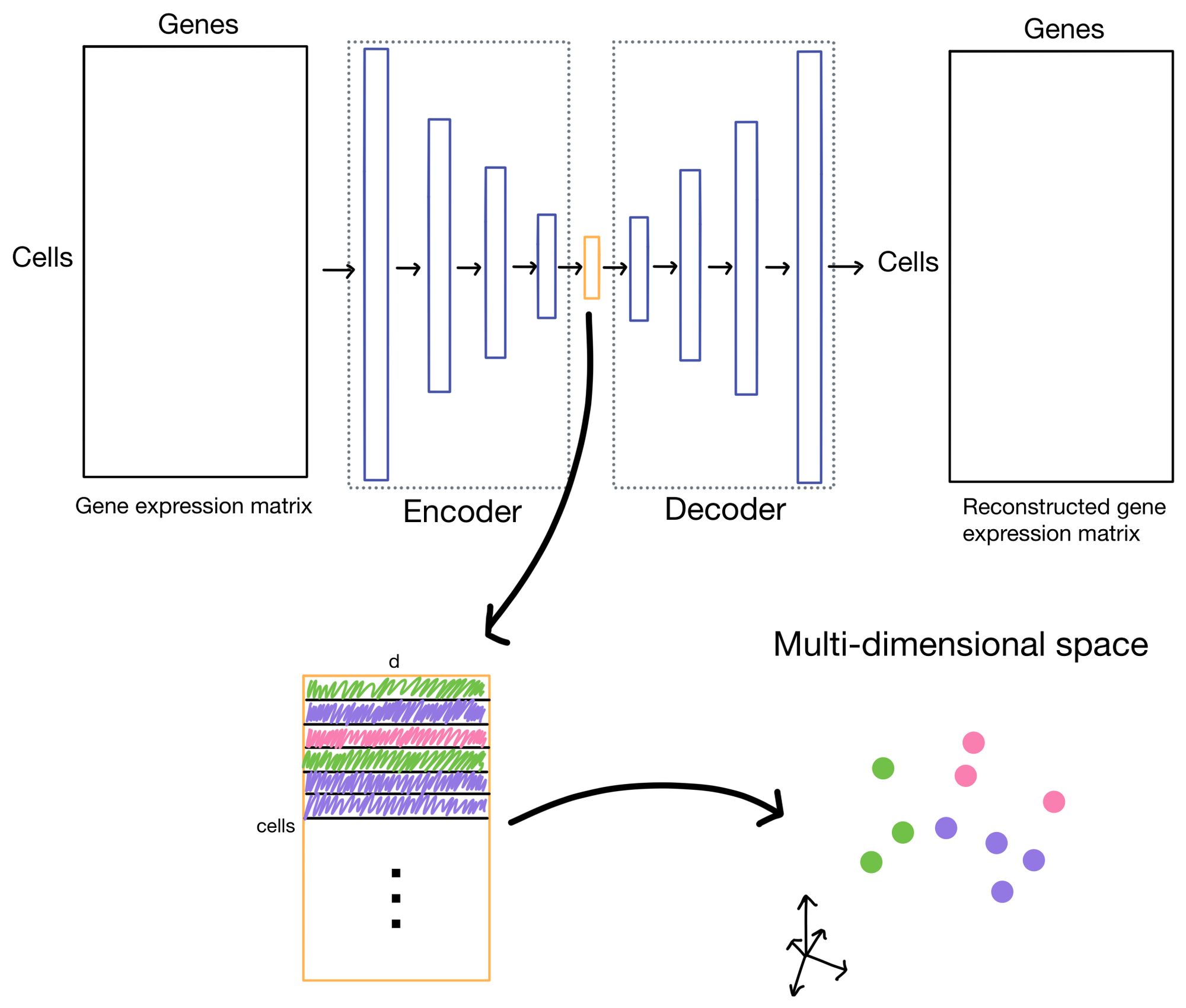
So what are autoencoders? Autoencoders are a flavor of neural network (shown below) in which the outputs of the network are reconstructions of the input. You can think of this almost as the ultimate "fake task". However, with autoencoders it usually isn't the outputs we're interested in, but hidden layer (also sometimes referred to as latent or embedding layer). This layer is purposely smaller dimensionality than the dimensionality of the input dataset (# of genes in the case of scRNA-seq data). This property forces the network to learn a condensed representation of the input data. Or in other words, the activations (outputs) of the hidden layer will be an information rich representation of the input data. In the case of expression data we can refer to these representations as cell embeddings.

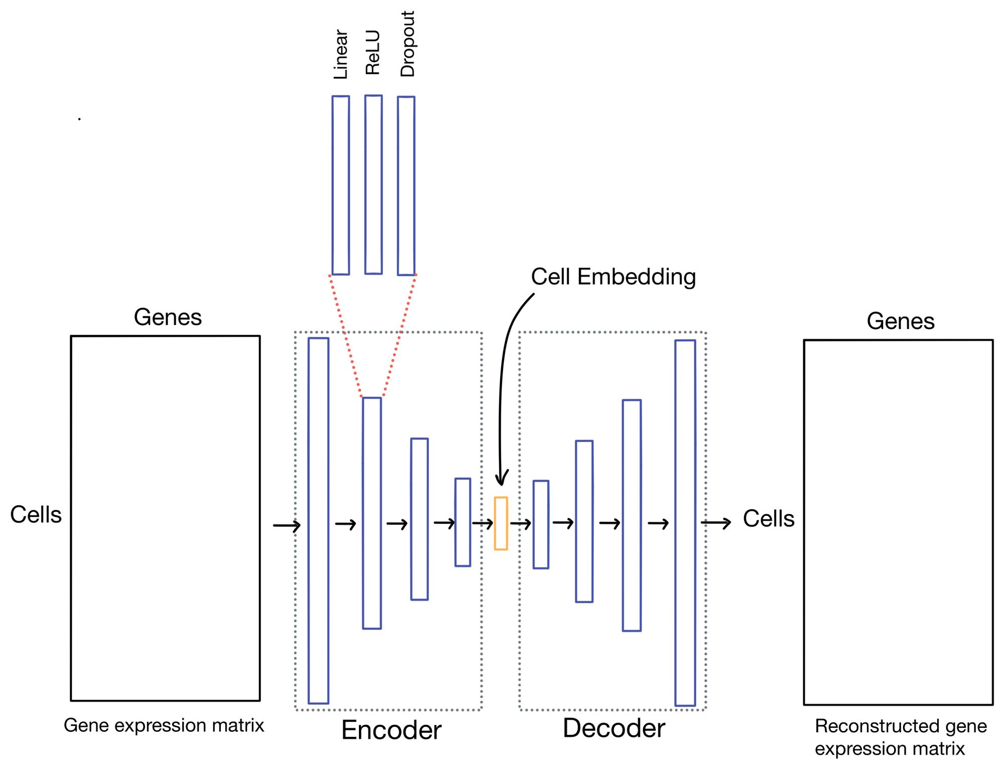
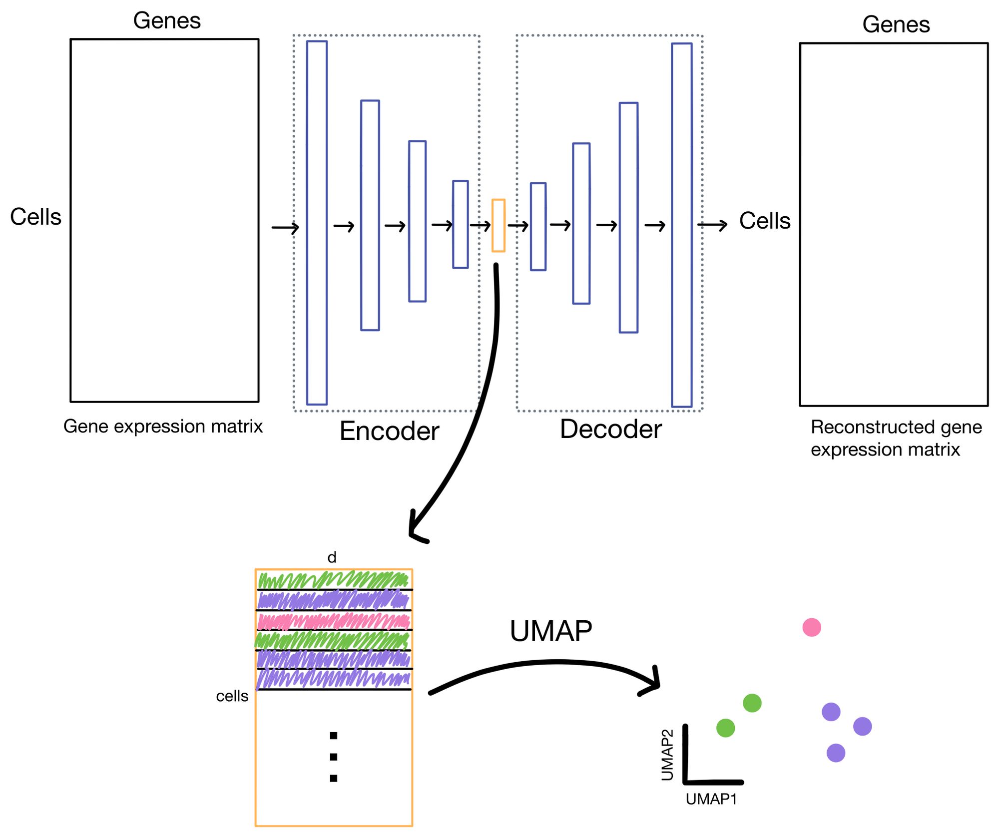
The cell embeddings, with dimensionality of d (where d << # of genes), is then used for downstream tasks such as clustering or low-dimensional visualization with algorithms like UMAP or t-SNE.

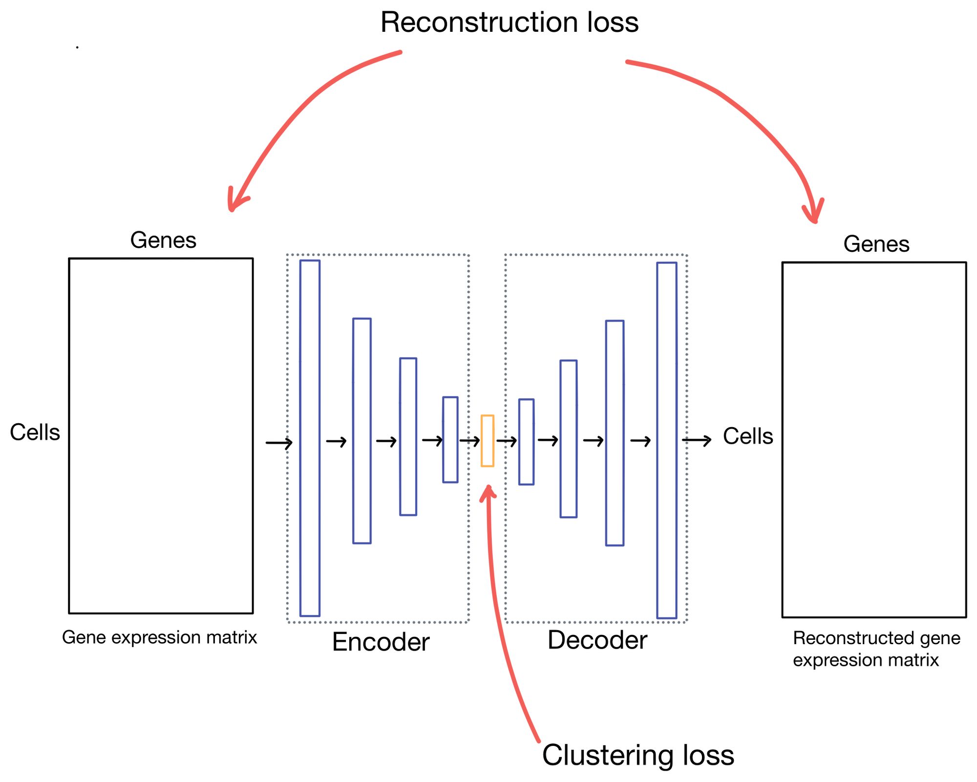
Stepping back to our autoencoder, in scDCC and DESC there are two different components to the autoencoder loss function: the reconstruction loss and the clustering loss. The reconstruction loss describes how well the outputs (which are reconstructions of the inputs) match the actual inputs, while the clustering loss measures how "well" the cells are clustering. As you can imagine there are many ways to describe how well a cell clusters, but for these methods, it's some formulation of "how similar are cells in a cluster to cells in the rest of the dataset".

This is also probably a good time to note that scDCC actually has a third component to its loss function that incorporates additional information about the single cell data, but I'll ignore that in this post as it's domain specific to the paper. Additionally, scDCC and DESC apply these loss functions in different parts of their training process and in slightly different ways (more on this later), but I will usually explain the loss functions in the context of a more basic autoencoder architecture for simplicity. So some parts of my explanation and diagrams may not line up exactly with what scDCC and DESC describe in their paper, but it should be close enough to get the point across.

Reconstruction loss

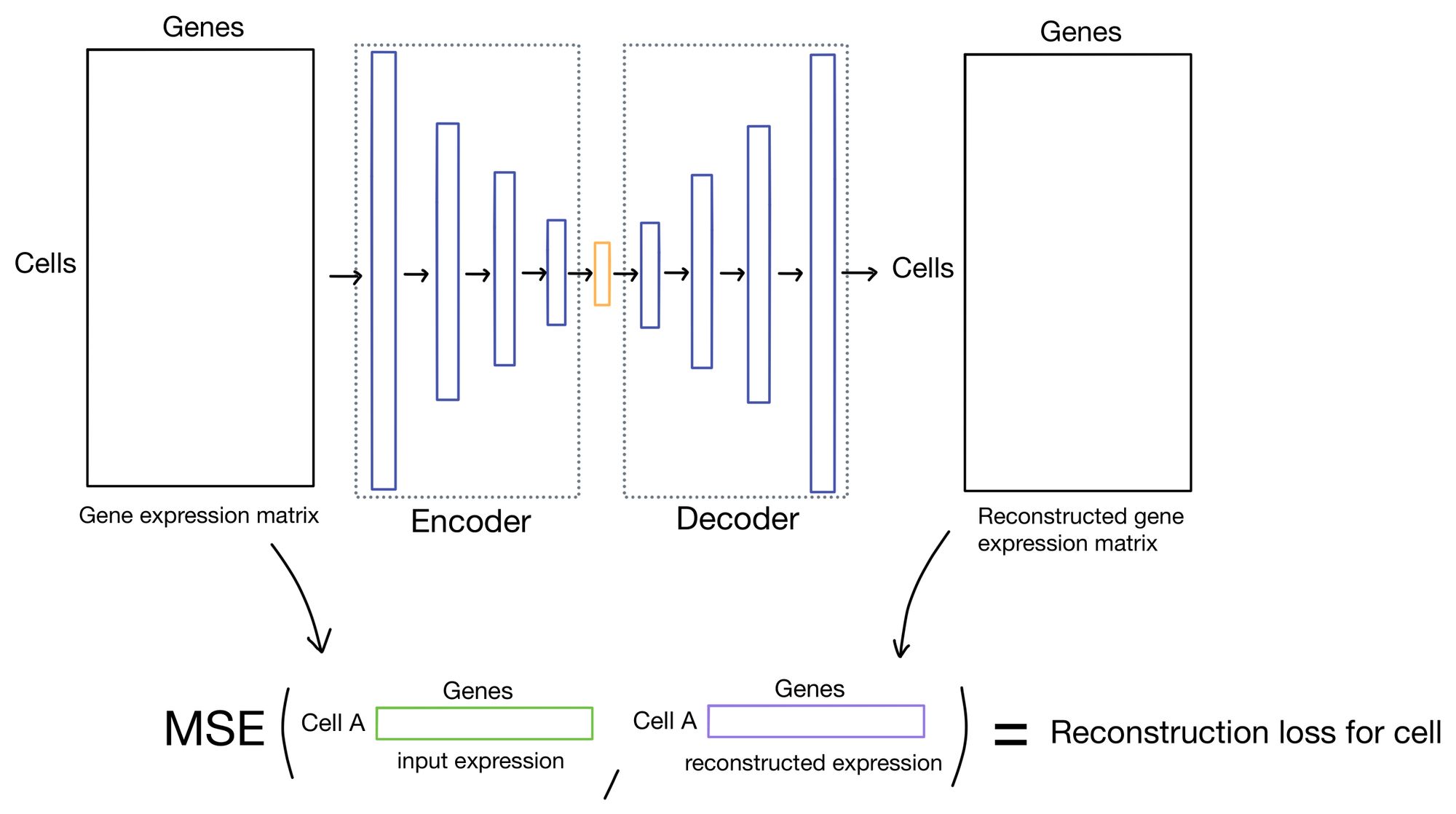
The reconstruction loss measures how close the outputs of the autoencoder are to the inputs. Typically this is done by taking the mean squared error (MSE) of the inputs and outputs. This is the approach that DESC takes.

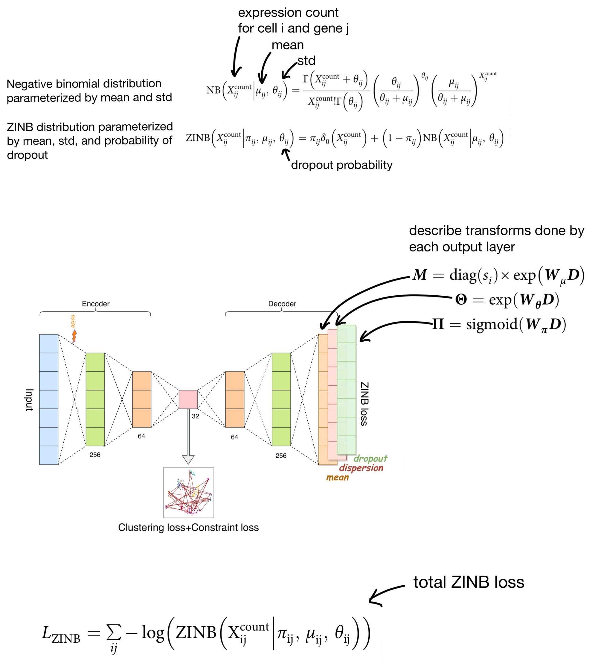
However, there has been some recent literature suggesting that using the zero-inflated negative binomial (ZINB) distribution is actually a better way of modeling single cell expression count data. The reasoning is that single cell data tends to be over-dispersed (meaning variance is greater than the mean) and suffers from dropout. The ZINB distribution takes care of modeling both of these issues, and is the approach scDCC takes for it's reconstruction loss.

The output of the ZINB distribution as the probability that a count of a given cell/gene came from a ZINB distribution parameterized by a certain mean, dispersion, and dropout rate. Meaning that in order to parameterize the distribution our network needs to come up with three outputs (mean, dispersion, and dropout) instead of just a single set of outputs, as you would need when using MSE as a reconstruction loss.

scDCC solves this by adding three separate output layers. The activations of these layers are then used to parameterize the ZINB distributions, which return the probability that a cell count was produced by said distribution. The ZINB loss function then attempts to maximize this probability by using the negative log likelihood of this probability as a loss function.

So that's one portion of the loss function, now we describe clustering loss.

Clustering loss

Before I get into the details of the clustering loss, it's worth noting that while DESC and scDCC apply the same clustering loss function, they do so in slightly different ways. DESC first trains the autoencoder by minimizing reconstruction loss only, and then remove the entire decoder portion of the network and trains exclusively on clustering loss applied to the the outputs of the embedding layer. scDCC, like DESC, will first pretrain the autoencoder solely on expression loss, but it will then incorporate clustering loss and reconstruction loss in the same overall loss function while it continues to train the network.

Before diving into the details of clustering loss, why do we need it in the first place? Let us take a moment to visualize the latent space (i.e. cell embeddings) of our autoencoder in multi-dimensional space.

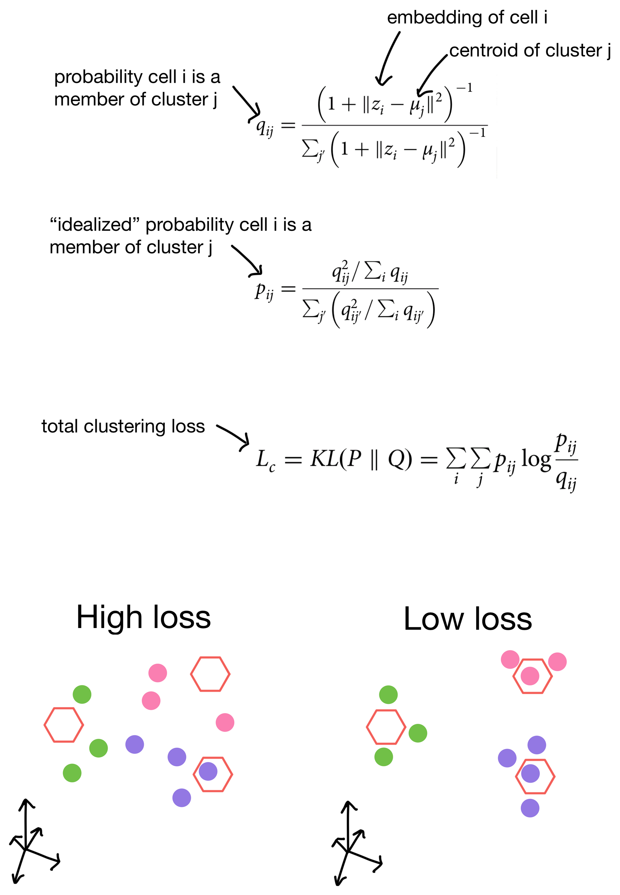
We want the cell embeddings to be as close as possible for similar cells, while being as far away as possible for differing cells. Imagine we have three clusters, whose centroids are represented by hexagons below. Ideally, our clustering loss function will drive the cells of the three clusters as close to the centroids as possible, and away from cells belonging to neighboring clusters.

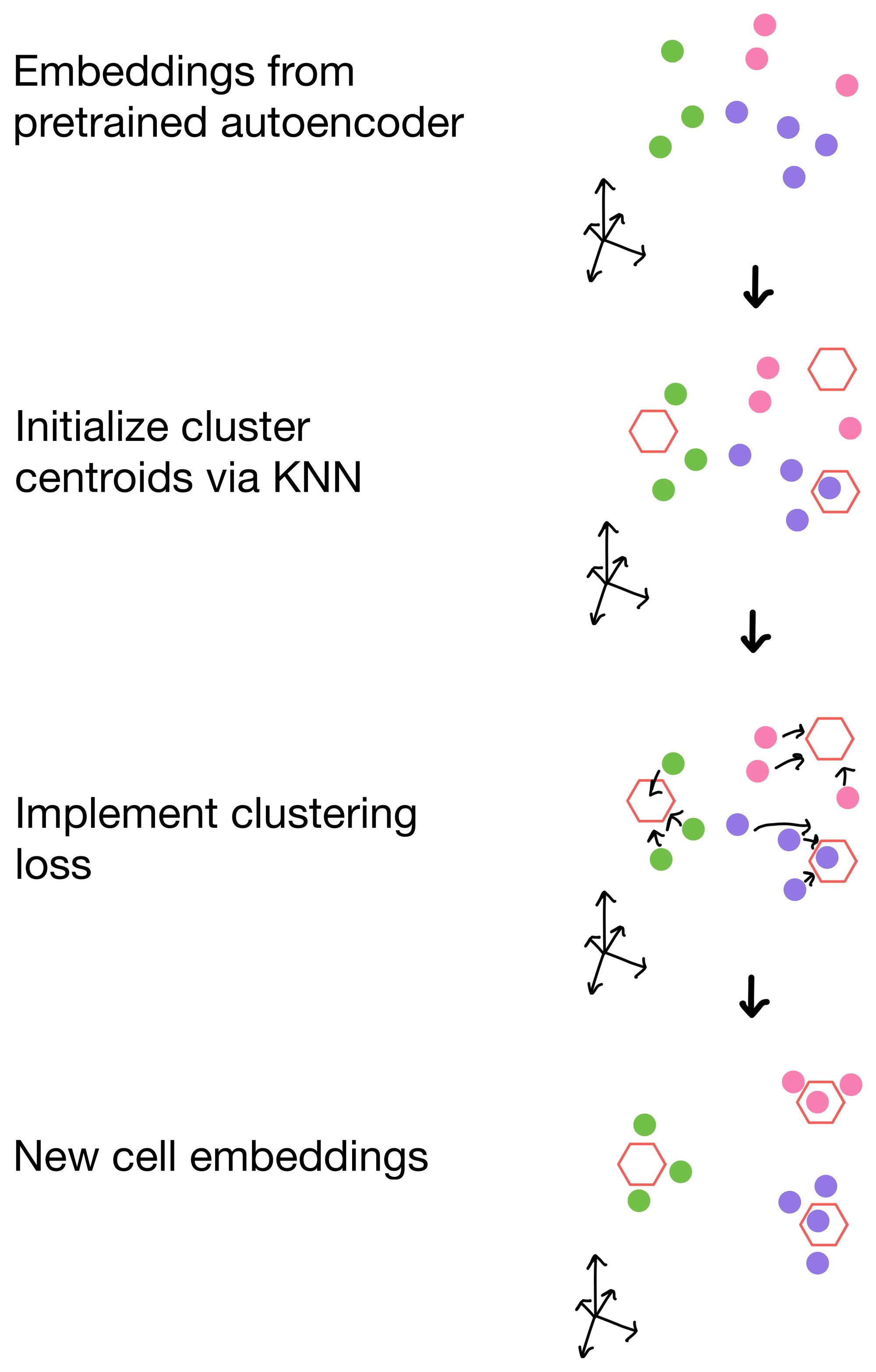
So how are these clusters initialized in the first place? For these methods, they are initialized from the cell embeddings generated by the pretrained autoencoders trained with only reconstruction loss. Then, when applied, the clustering loss function will drive the cells to aggregate around the centroids of these clusters.

The student's t distribution (first used for this type of clustering purpose in t-SNE), is used to measure similarity of a cell to a given cluster. In other words, the probability that a cell belongs to each cluster. This distribution is termed q. We then construct an "idealized" version of q that we call p. p is essentially just a sharpened version of q, meaning that cells that already have high probability of membership to a cluster will have even higher probability of membership, while clusters that are farther away will have even lower similarity scores. The total clustering loss is obtained by taking the KL divergence (a method for measuring the similarity of two distributions) between p and q. This has the effect of pushing q towards the idealized distribution p. Over the course of training this, in theory anyways, will result in better clusters.

So by including clustering loss in the overall loss function for the network we're more likely to see these nice properties in the cell embeddings generated from them.

There you have it, how autoencoders can be used to obtain cell embeddings with idealized clustering properties.

Hope you enjoyed the post. Cheers :)

1. DESC: https://www.nature.com/articles/s41467-020-15851-3
2. scDCC: https://www.nature.com/articles/s41467-021-22008-3
3. scGen: https://www.nature.com/articles/s41592-019-0494-8
4. scvis: https://www.nature.com/articles/s41467-018-04368-5