Explainer: CNNs and ResNets - Part 2

First, before we begin, if you aren't already familiar with convolutional neural networks (CNNs), check out part 1 of this post here. There I cover the basics of 2D convolutions and build an intuition for how CNNs work.

In the paper Deep Residual Learning for Image Recognition ^[1], He et al. introduced the ResNet architecture, which at the time was a big step forward in terms of performance for convolutional neural networks. Most of the performance gain came from the introduction of residual connections, which I cover in more detail later in the post. These connections allow for input signals to propagate further through the network than they otherwise would. This feature allows for the training of deeper models with more layers CNNs at the time.

First, a refresher.

Below is a schema for a basic-ish convolutional neural network.

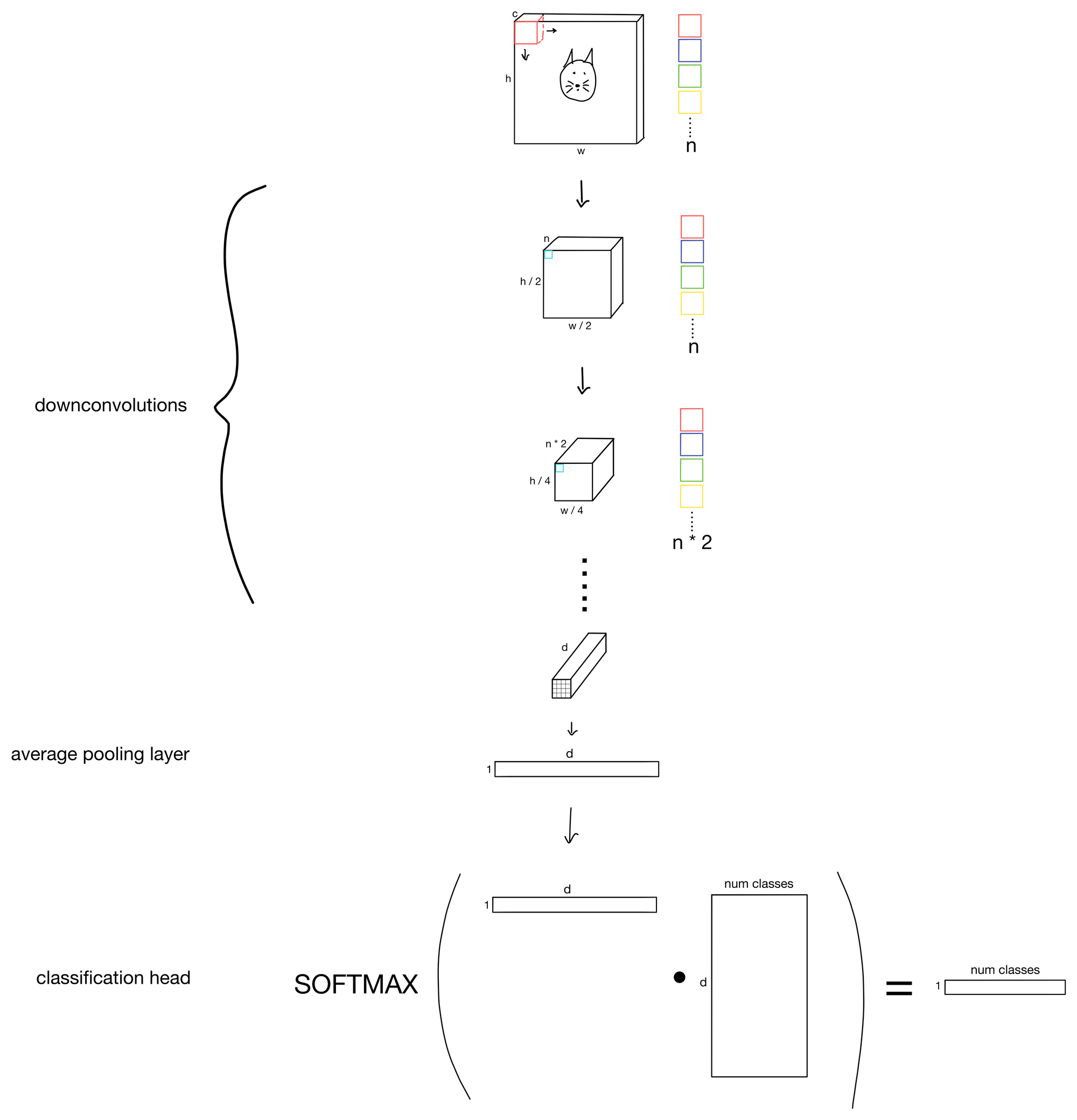
We start from a traditional 3-channel RGB image, and slowly, through the addition of more more and more channels (i.e. increasing the number of features maps), and the reduction of kernel stride (i.e. downsampling the height and width dimensions) we obtain increasingly rich representations of the input. Then we simply attach a head to the network to achieve whichever task we desire.

ResNets follow the same general principles, but with a twist.

Residual Connections

The major contribution of the resent is the residual connection (sometimes referred to as skip connections). Surprisingly, all a residual connection does is simply add the input of a layer block to the output. Depending on the total number of layers in the ResNet (there are several ranging from 18-152) the parameters of the convolutional layers that make up the block may be different, but all blocks follow the same general pattern shown below.

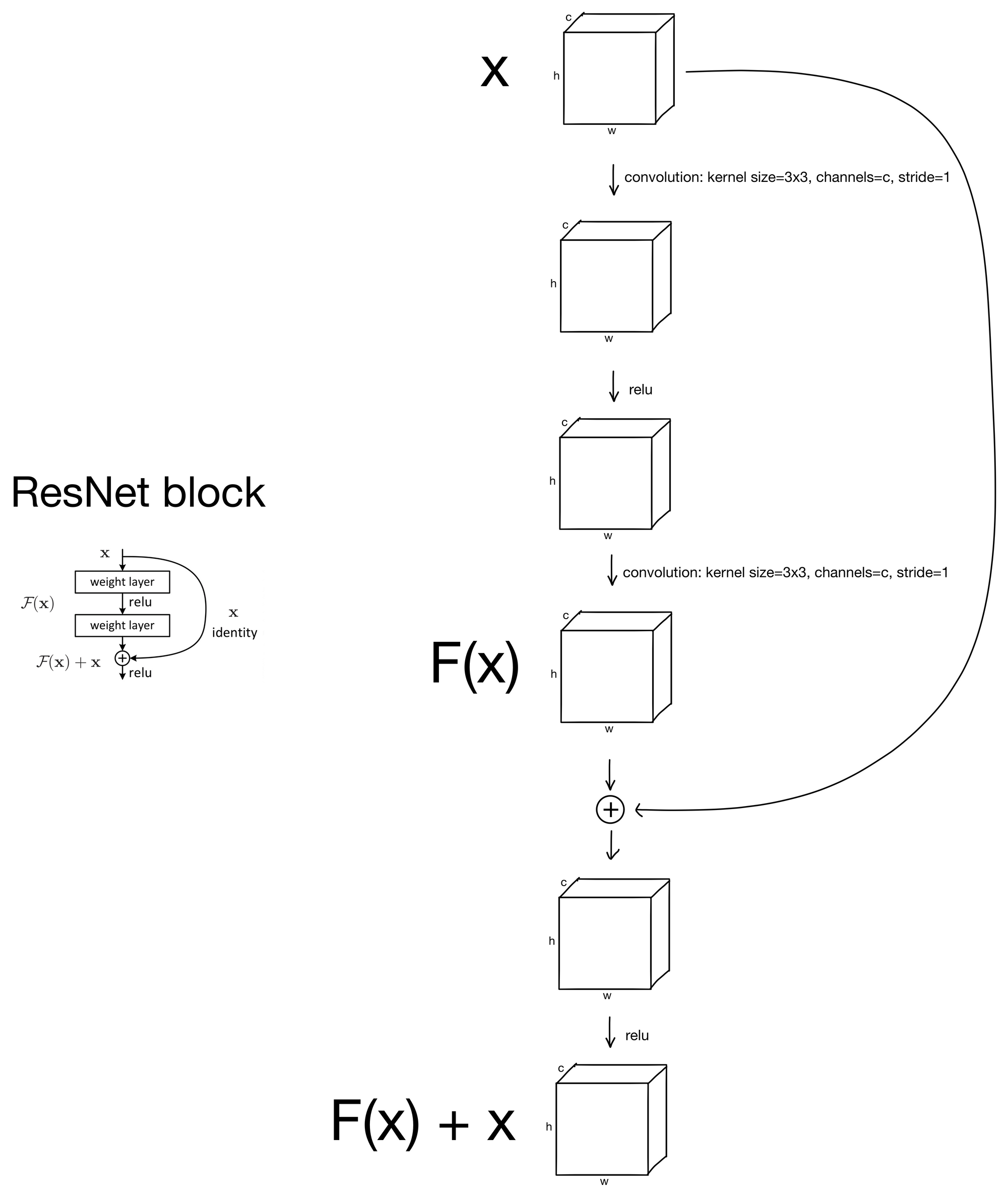
As you can see, all there is are some convolutions, after which the block input is added to the output prior to a final RELU activation function.

That's it! Surprisingly simple.

So how are these ResNet blocks arranged in the network? Below is a 34-layer ResNet with a block shown in more detail. All the blocks with solid lines (representing the residual connections), follow this same structure, just with differing numbers of channels.

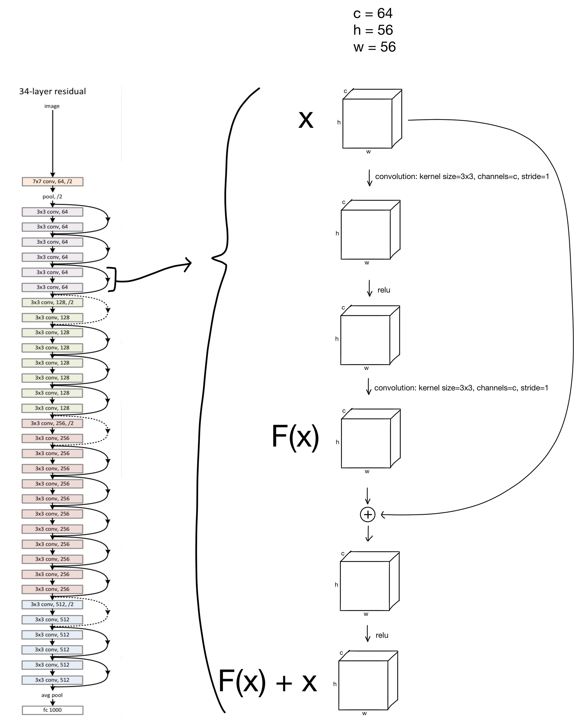
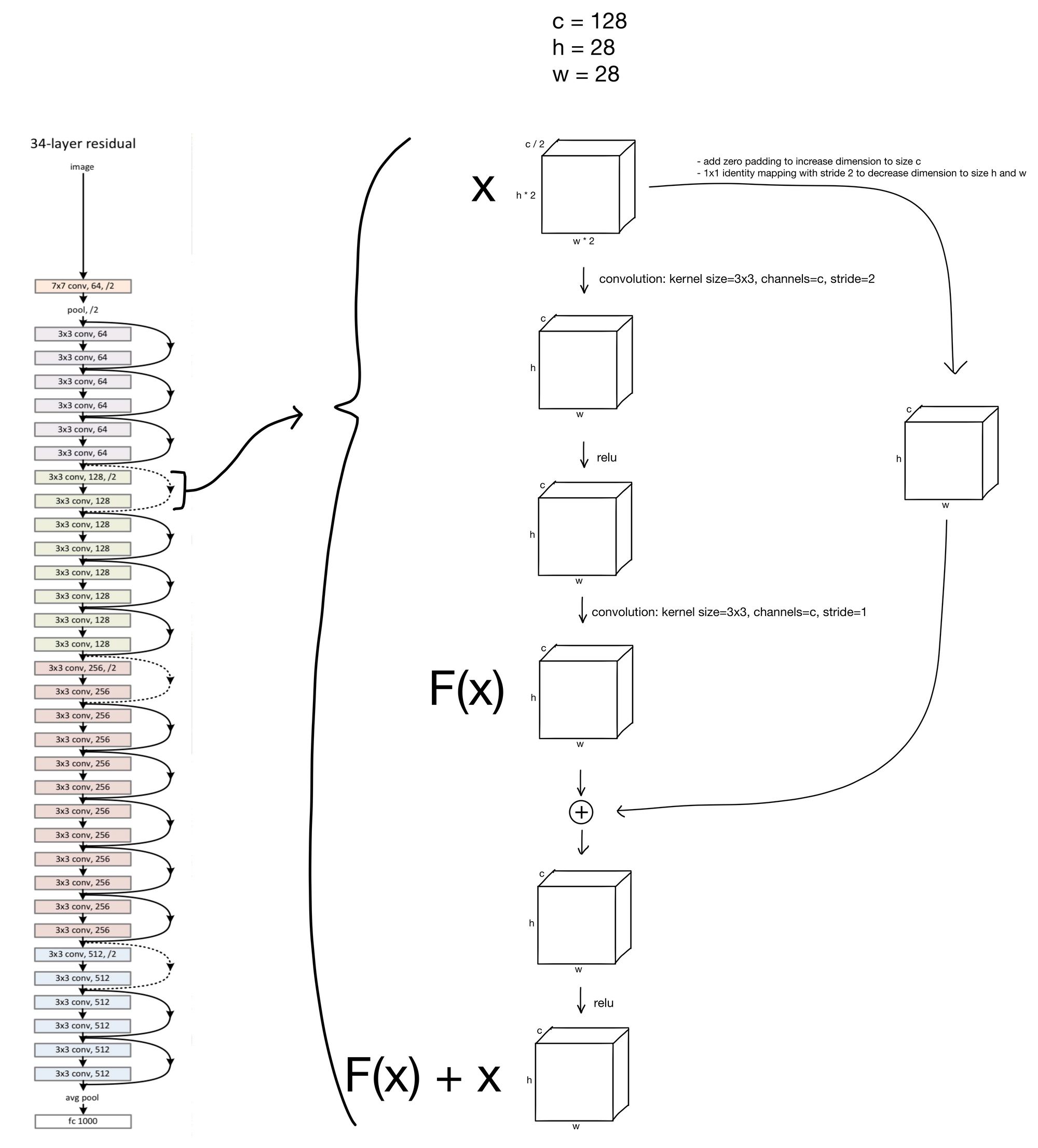
You may have noticed that the residual connections in the schema are either dashed or solid. The solid lines are residual connections for layer-blocks with identical input and output dimensions, which is what we've previously shown. So what about the dashed lines? These are somewhat special cases for the residual connections. You'll notice that the first convolution in these blocks have a stride of 2 while increasing the number of channels by a factor of 2. This creates somewhat of an issue, as due to this downsampling the inputs of the block no longer will match the outputs, making them impossible to add together.

The authors tried multiple methods to remedy this mismatch. The first, A) was simply to add zero padding to address the increase in channel dimensionality, and perform an identity (meaning no change to the input) 1x1 convolution with a stride of 2 to address the decrease in feature map height and width. The second option B) was to use weights to project the input, via 1x1 convolution with stride 2, to match the new channel dimension. The authors found B to be slightly better, but not enough of an improvement to justify addition of the extra parameters and complexity, so they stuck with option A (shown below).

Bottleneck ResNet Blocks

The authors make one more small modification only for deeper architectures (> 34 layers). In these deeper networks the authors add bottlenecks to the layer blocks to decrease the total number of parameters, thereby allowing for improved training efficiency.

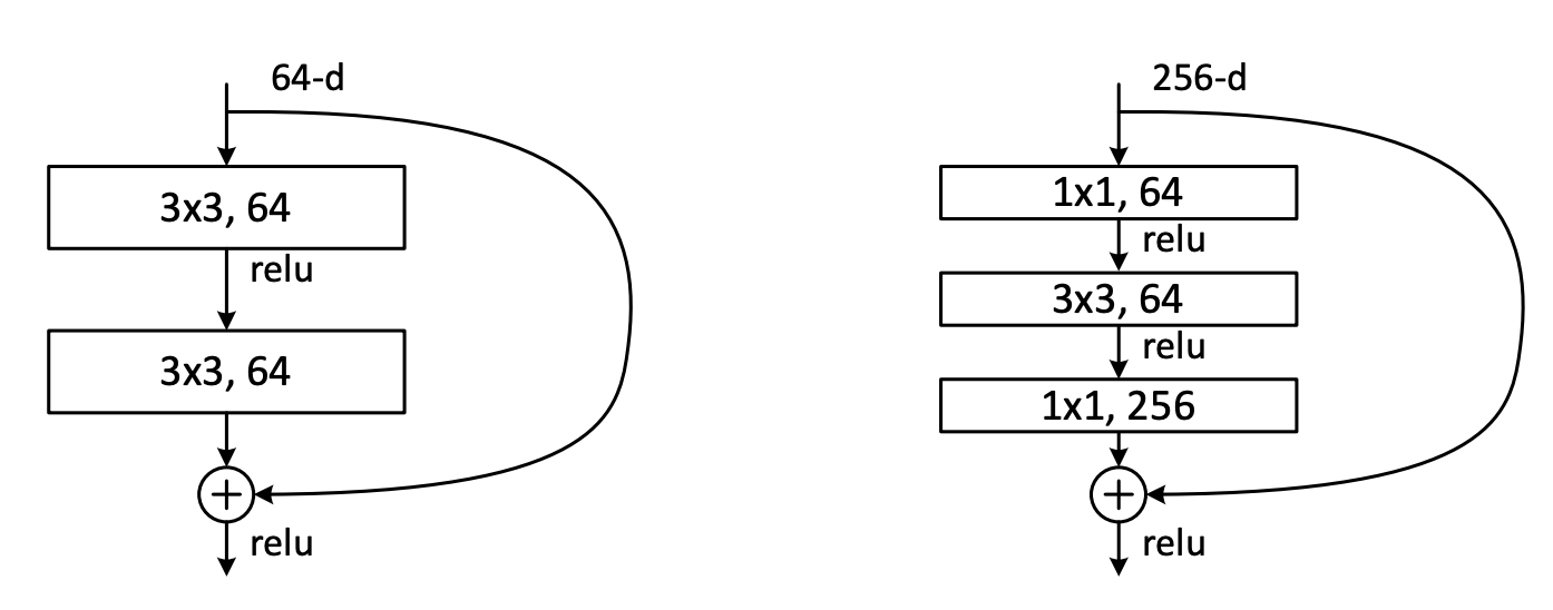
Residual connections are especially important in this case, because with the bottleneck information is lost from the block input, but the residual connection allows for that information to be added back in after the channel dimension is projected back to original size.

There you have it, ResNets. Hope you found the post useful :)

1. ResNet: https://arxiv.org/abs/1512.03385