Explained: Principle Component Analysis (PCA)

In this post, I'll cover principle component analysis (PCA). The motivation behind principle component analysis is that you can reduce the feature space of a dataset such that after the reduction we are left with a smaller number of new features that are effectively a compression of all the information in the old features. This is useful in a variety of contexts, usually where there is a high dimensional dataset (where the number of features is very large, or much larger than the number of samples). In these datasets PCA condenses the dataset to simplify the "patterns" in the dataset to a smaller number of features, which can help with downstream analyses.

We start with a dataset A (of shape n_xd) with n samples and d features.

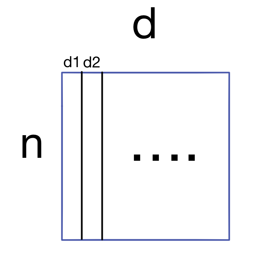
The first step is to generate the covariance matrix for A.

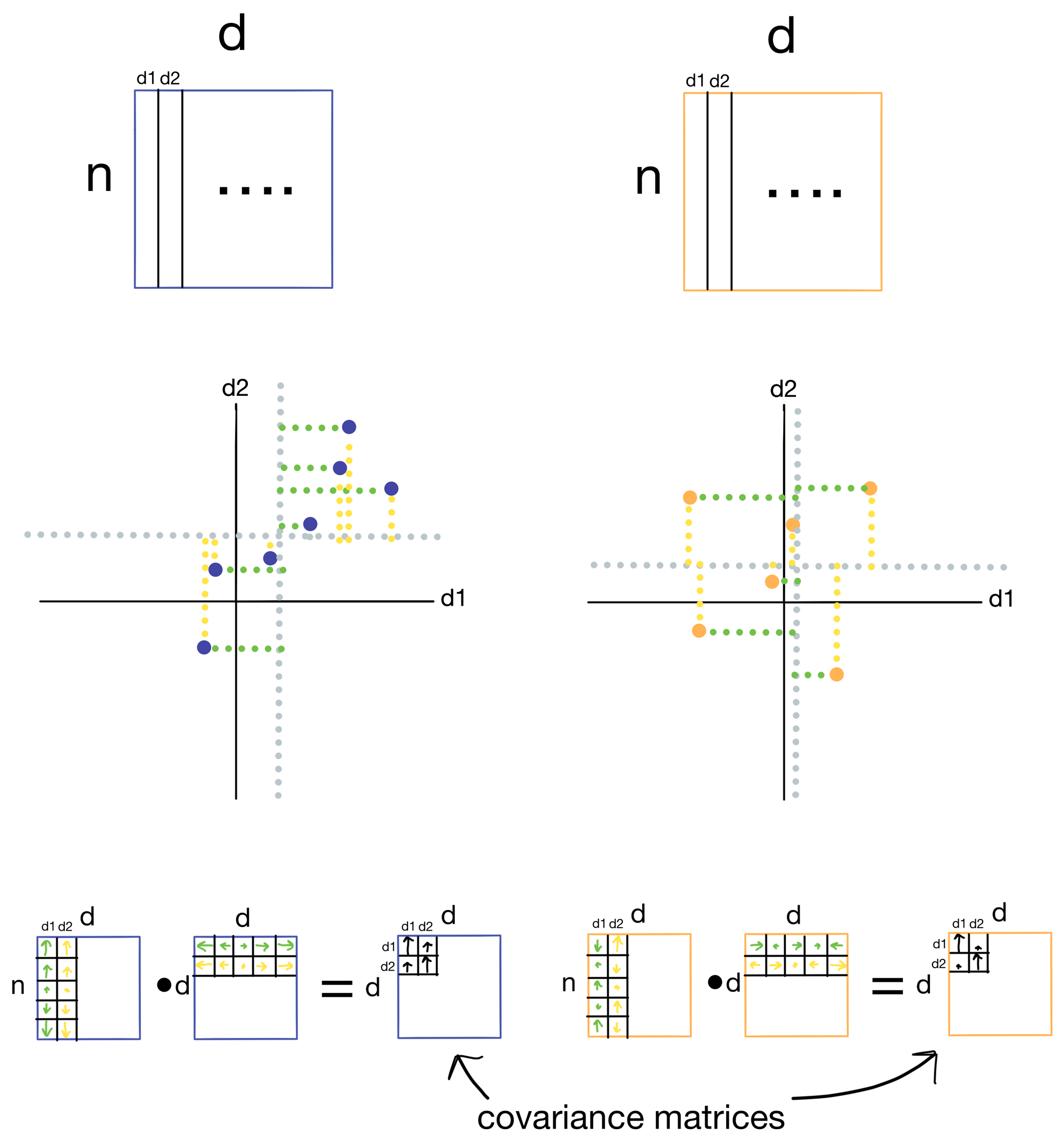
1) Covariance Matrix

Below is an example of the construction of separate covariance matrices for two datasets: 1) our example dataset A where the first two features d1 and d2 are highly correlated, and 2) another dataset where the first two features d1 and d2 are not well correlated.

Covariance is a measure for how well two features vary with each other (think of it as an unnormalized version of correlation). Two features that vary in the same way will have high covariance, and two that don't will have low covariance. To calculate the covariance matrix we take the dot product of the residuals, which are the distances of each of the samples from the mean for a particular feature. Residuals for d1 are shown in green and residuals for d2 are shown in yellow for each sample (i.e. point) in the dataset. When the samples have residuals that tend to be in the same direction and magnitude, we get large covariance (blue), however, when they are not we get low covariance (orange). In the resulting covariance matrix each entry is the covariance for a given pair of features.

Now that we have a covariance matrix, we can derive the principle components of our dataset via eigendecomposition.

2) Eigenvalues and Eigenvectors

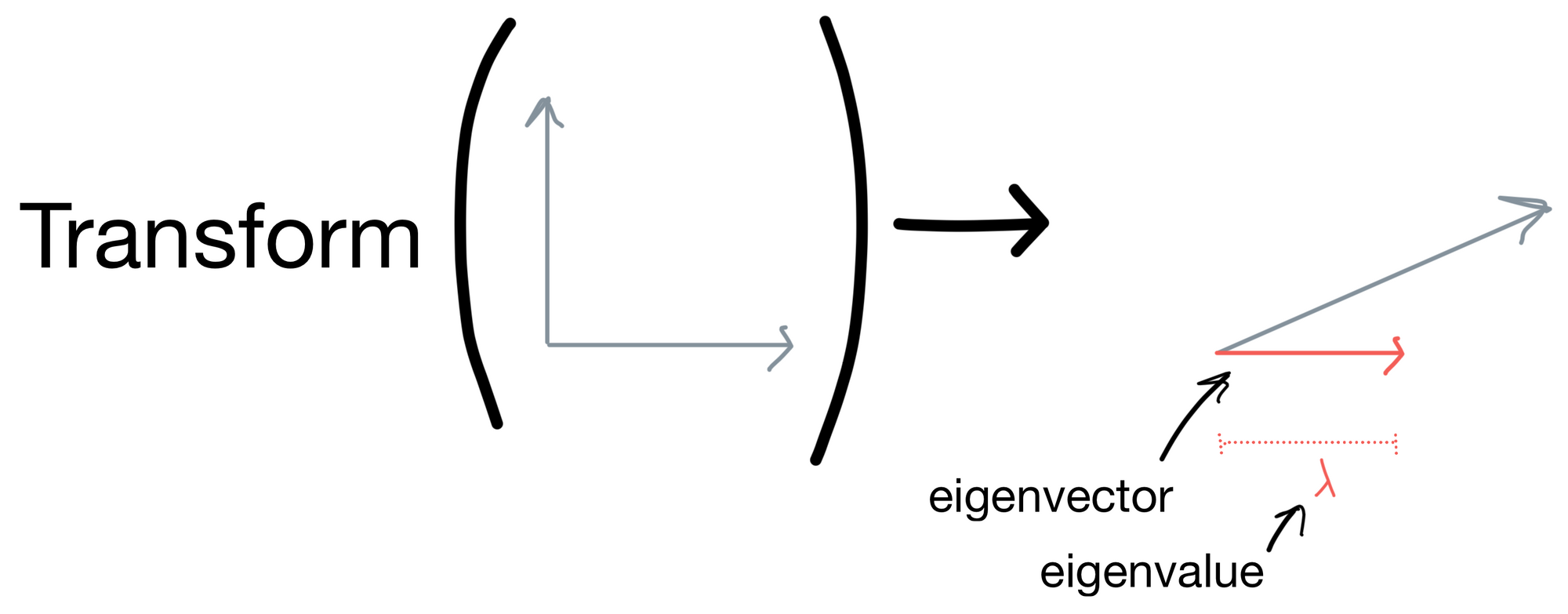
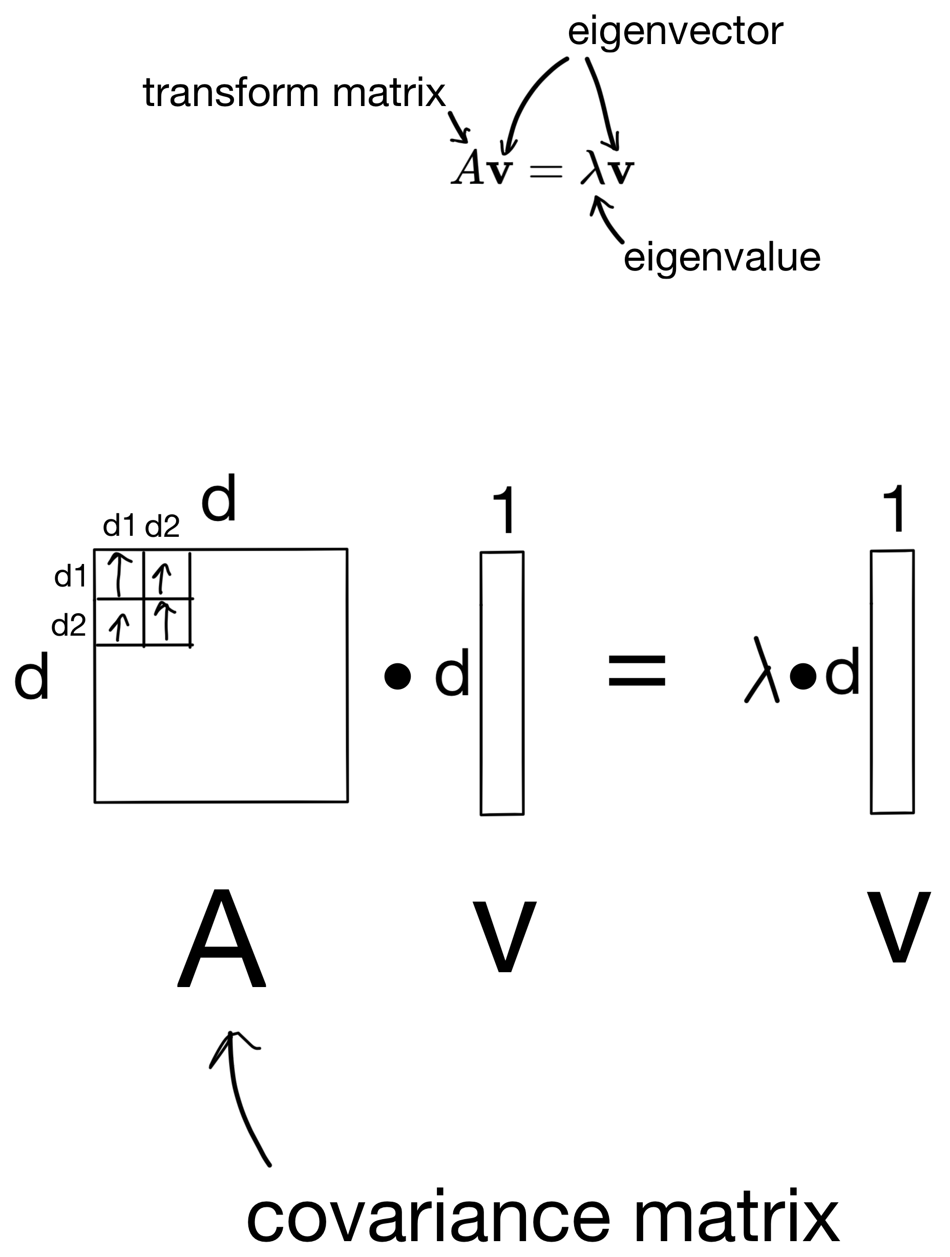
Via wikipedia, an eigenvector is defined as "a nonzero vector that changes at most by a scalar factor when that linear transformation is applied to it" and the eigenvalue is "the factor by which the eigenvector is scaled".

Let's get come intuition for this definition. Below is a set of vectors that have some transform applied to them. After the resulting transform they are stretched in some direction. The eigenvector is vector for which the direction stays the same (shown in red). The eigenvalue is the magnitude of this eigenvector.

In the case of our covariance matrix, you can think of the eigenvectors as the direction in which the covariance matrix would stretch a matrix if it was applied as a transform, and eigenvalues would be the magnitude of that stretching. This sounds a lot like what the principle components are, given they are the directions representing the most variance in our dataset. In fact, the resulting eigenvectors are the principle components of the dataset the covariance matrix was derived from, and the eigenvalues are the importances of the principle components (i.e. how much information the principle component carries).

So how are these eigenvectors and eigenvalues derived? First, we start with the below equation, where we use the covariance matrix to transform a basis vector (i.e. eigenvector), such that the result is equivalent to some scalar (the eigenvalue) multiplied by the basis vector.

I wont go into the details, but we can then derive the eigenvalues by solving some linear equations (shown below).

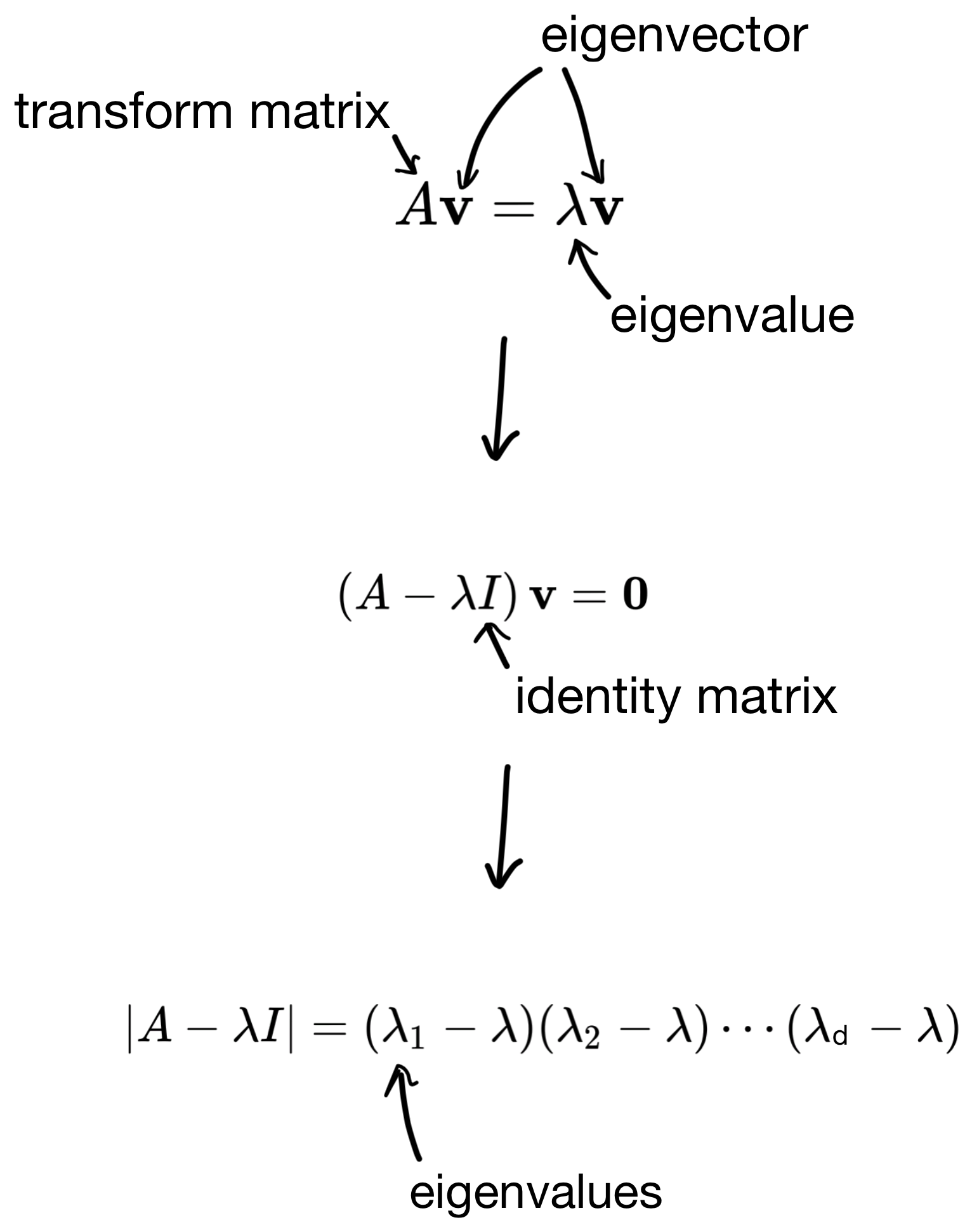
And then plug the eigenvalues back in to get the eigenvectors. The number of solutions to the equation is equivalent to the number of features in the dataset (i.e. the dimensionality of the covariance matrix). So in the end we end up with d eigenvector/eigenvalue pairs.

3) Putting it all together

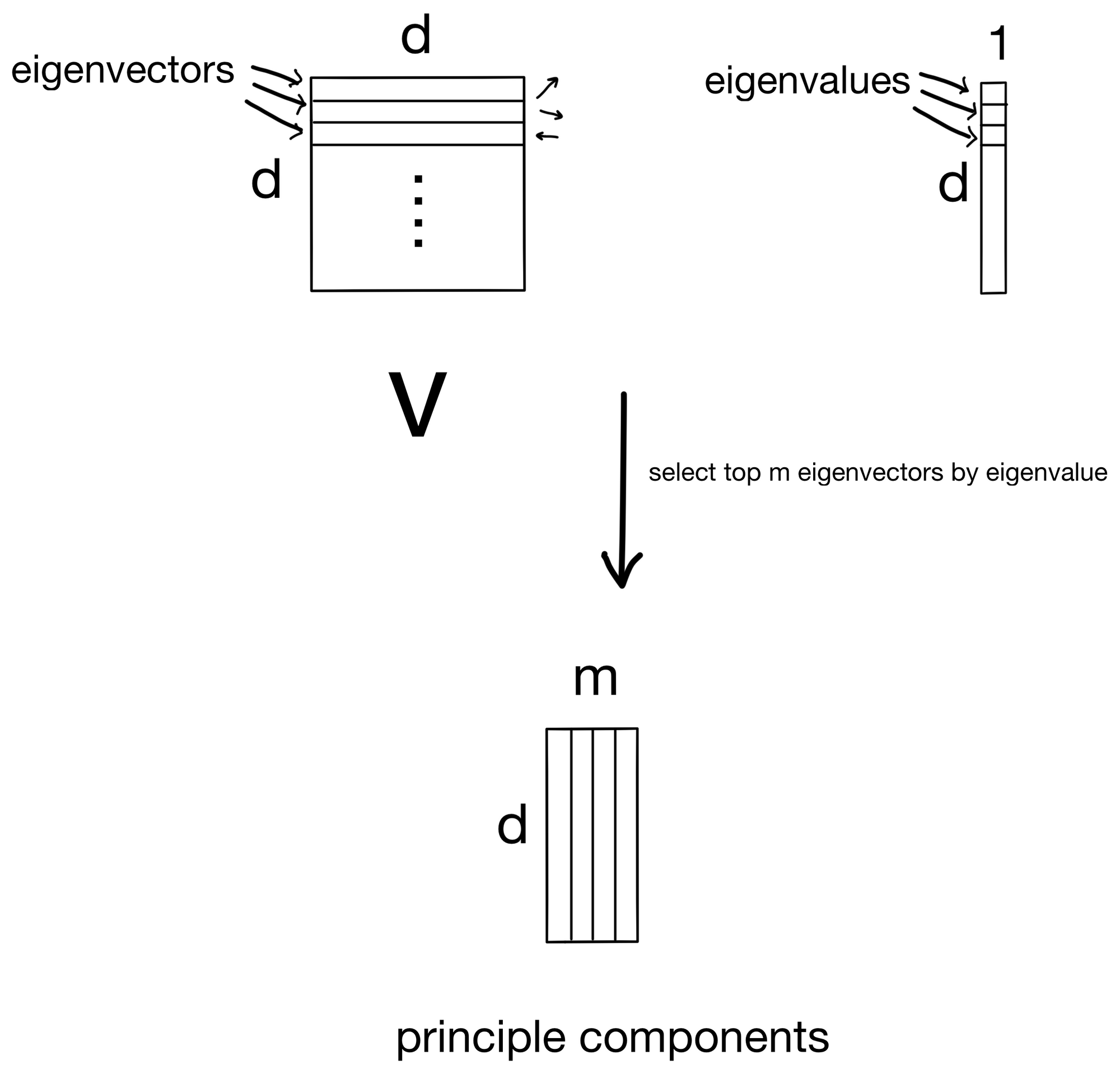
Since the eigenvectors are the principle components, we simply rank them by eigenvalue (the importance for its given principle component) and select the top m components to keep.

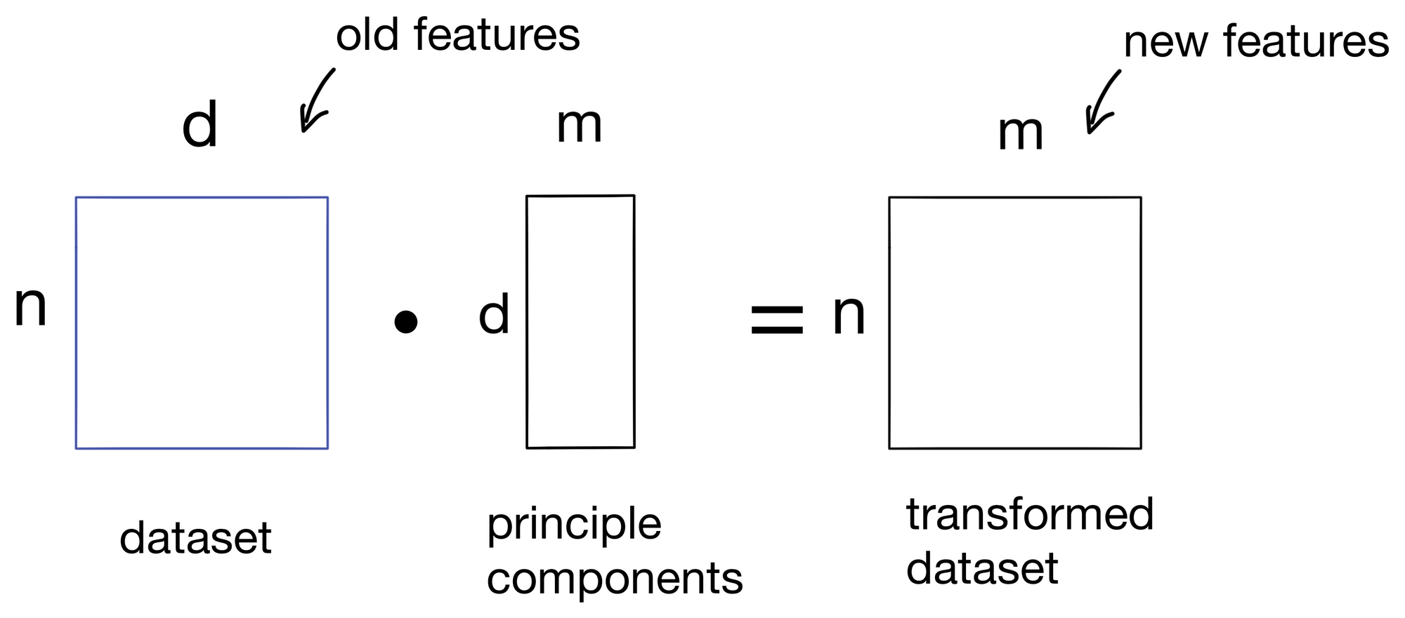
These components are then used to transform our initial dataset into a new dataset with m features, one for each principle component. We now have our transformed dataset!

Hope you found the explainer useful. Cheers :)