Explainer: Convolutional Neural Networks (CNNs) - Part 1

This post is a two parter, where in next weeks companion post I'll cover the classic paper Deep Residual Learning for Image Recognition^[1], which introduced the widely used ResNet architecture. Although transformer-based architectures have recently begun to transplant convolutional neural networks in many imaging tasks, they still perform competitively, and can even can be incorporated into transformer architectures to form hybrid architectures that outperform each architecture individually^[2].

Current reasoning as to why convolutional networks are so effective is that they have an inductive bias towards image-based tasks.

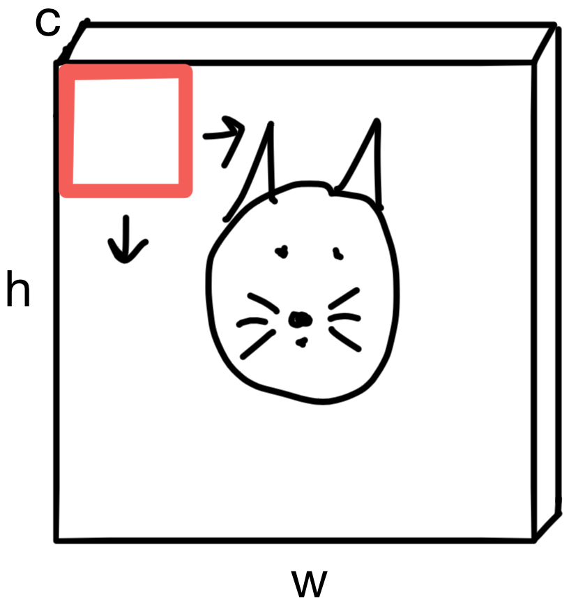
Take for example this poorly drawn picture of a cat.

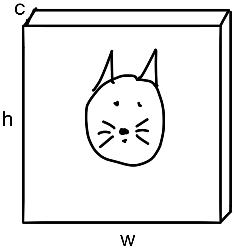
If we randomly selected a region of the image, say a portion of the image containing the cats ear.

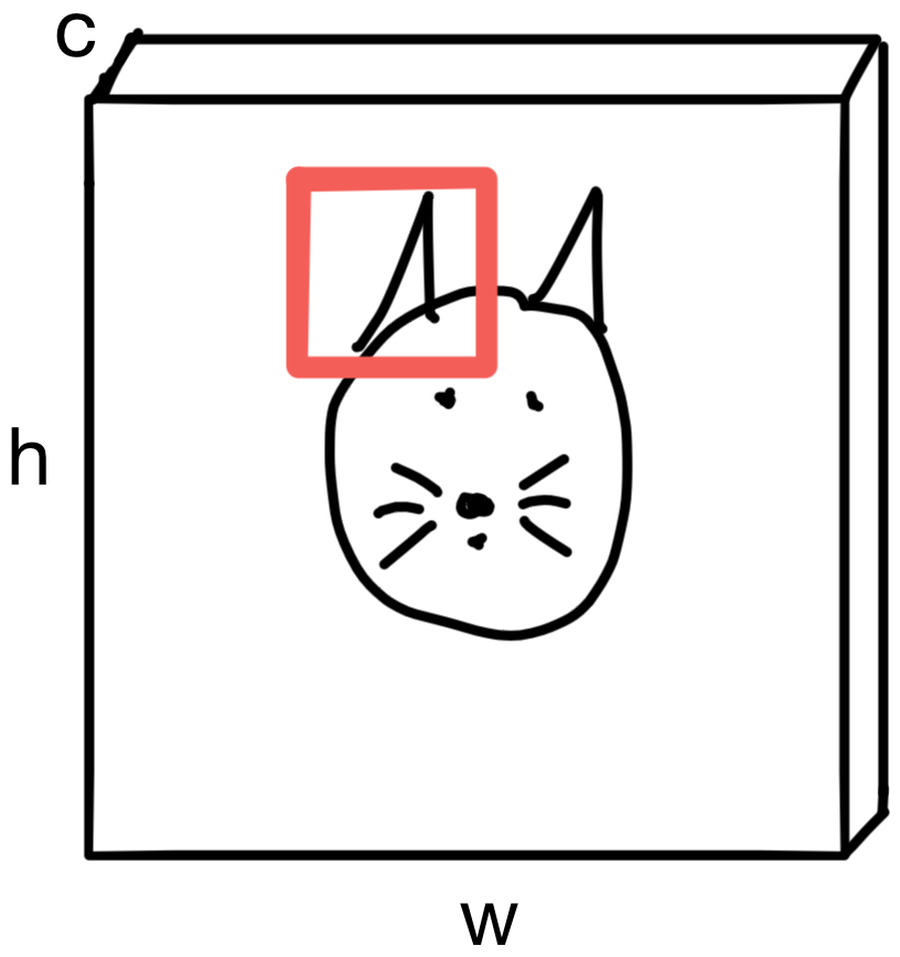
The pixels in the region carry spatial context. In other words, pixels in that neighborhood are more likely to be "ear" pixels than pixels in a different region of the image, which may be "whisker" pixels.

Convolutions take advantage of this spatial relationship by iteratively building up representations of the input image that carry more and more context of the entire image. Until eventually, the network can "see" the entire image.

So how do convolutions build up these representations?

Convolutions

Kernels matrices (sometimes referred to as filters) are the basic building blocks of a convolutional layer. More details later, but for now the basic idea is that each convolutional layer consists of multiple learned kernels that are responsible for extracting various types of representations from the image. For example, one kernel may extract top edge boundaries, while another may do right edges, etc.). As we go further down the network the representations these kernels gradually become more complex. In early layers, the network detects edges and simple shapes, while in later layers more complex concepts like faces, or in a cats whiskers, are seen.

How do kernels help build these representations?

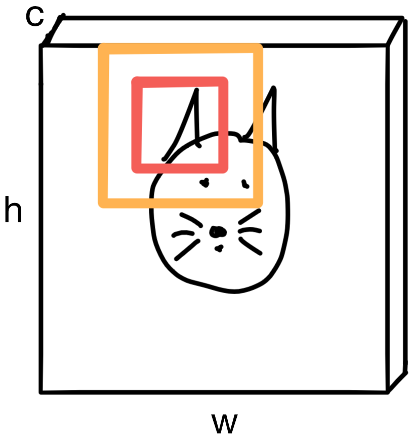
To build representations, each kernel (shown in red) is "slid" across the image. The amount a kernel is "slid" is called the stride of the convolutional layer. If a stride is 1, then the kernel is shifted by 1 pixel across the image, while for a stride of 3 the kernel would shift by 3 pixels across the image.

What type of operation do the kernels actually perform?

For each kernel, each pixel in region of the image the kernel is aligned with is multiplied by the kernel weight matrix (size k by k, where k is the height/width in pixels of the kernel matrix). For multichannel images, the kernel is applied to each image channel. The resulting values are summed to a single scalar value. This operation is performed everywhere the kernel is slid, eventually building up a feature map.

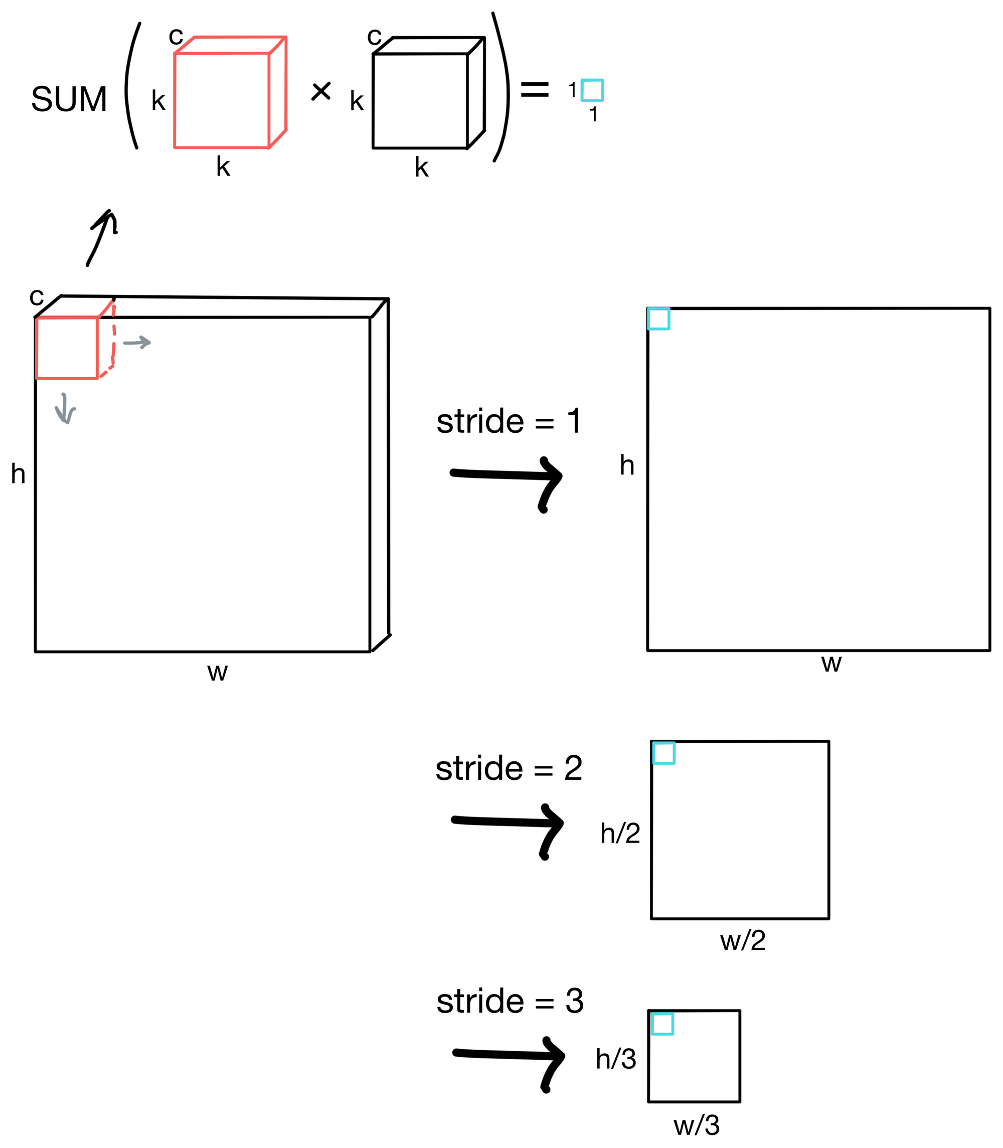
As you can see from the above figure, by increasing the stride we can also downsample by decreasing the heigh and width dimensions of the feature maps. By downsampling and continuing to keep the kernel size the same through consecutive layers of the network, we allow the network to see larger and larger regions of the image and increase its receptive field.

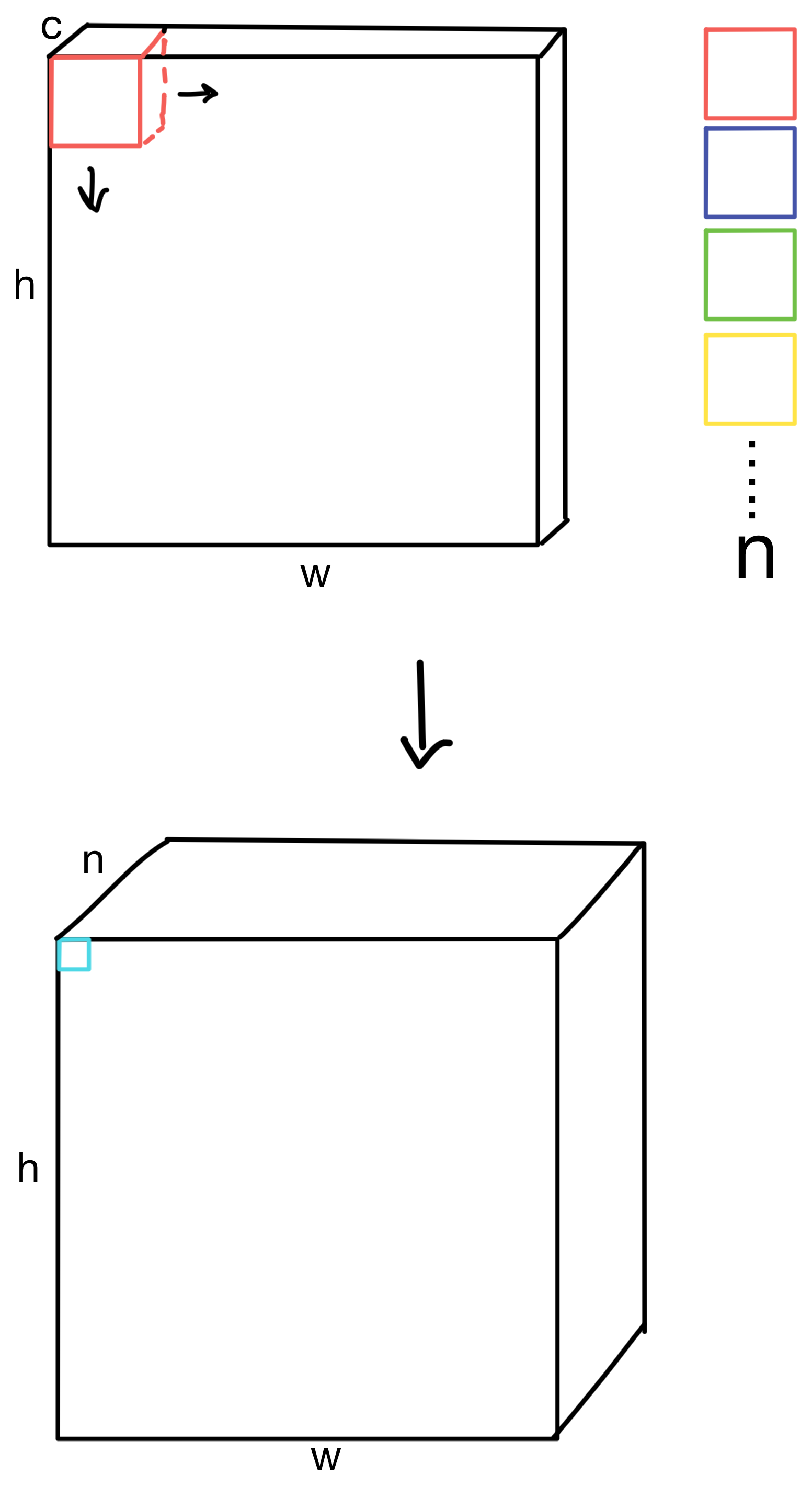
CNNs typically downsample by increasing the stride of a layer while simultaneously increasing the number of kernel matrices (i.e. filters) for various layers in the network.

Typically this is done repeatedly until the height and width dimensions of the feature maps are relatively small (for example 4x4 or 8x8). At the deeper layers of the network, we theoretically now have a rich representation of the image, which is useful for downstream tasks.

An example CNN

For example, to perform image classification, we would do an average pooling layer (where each of d feature maps is averaged to a single value). The resulting tensor would be passed through a classification head to produce a probability vector with the number of classes we are tasked to predict. An example of such an architecture is shown below.

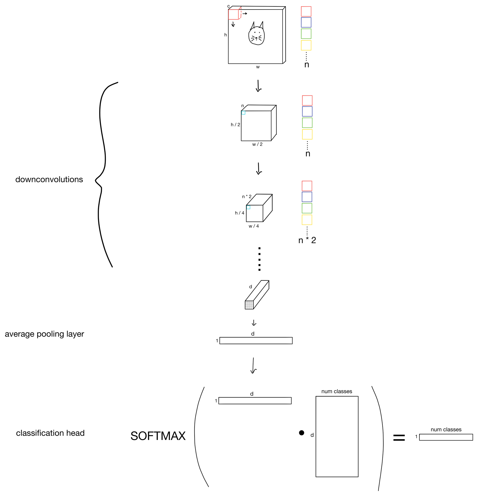
Top performing convolutional networks are of course slightly more complicated than this simplified network. Though they do tend to use all the same building blocks discussed in this post, and aren't too drastically different than the above simplified architecture.

Next week I'll cover the popular ResNet architecture, which, though slightly outdated now-days, was a seminal improvement for convolutional neural networks at the time of its release.

1. ResNet: https://arxiv.org/abs/1512.03385
2. Early Convolutions Help Transformers See Better: https://arxiv.org/abs/2106.14881