Explained: Multi-head Attention (Part 1)

Transformers have become nearly ubiquitous for a variety of machine learning tasks. In general, the feature responsible for this uptake is the multi-head attention mechanism. Multi-head attention allows for the neural network to control the mixing of information between pieces of an input sequence, leading to the creation of richer representations, which in turn allows for increased performance on machine learning tasks.

In part 1 of this multipart post, I'll cover the attention mechanism itself, and build an intuition for the why and how attention works. In part 2 next week I'll cover multi-head attention and how it is put to use in transformer architectures^[1,2,3].

Attention

The key concept behind self attention is that it allows the network to learn how best to route  information between pieces of a an input sequence (known as tokens). For example, if we take the sentence the cat jumped over the lazy dog, we would expect the network to learn to associate cat with jumped and lazy with dog (for more on attention for natural language processing (NLP) tasks see my post here). Attention applies to any type of data that can be formatted as a sequence. For instance, it can also be used with imaging data, where typically an image is represented as a sequence of patches that are then used as tokens in a sequence (more details on vision transformers in my post here).

So after all that, what's the equation for the attention operation?

Attention Equation

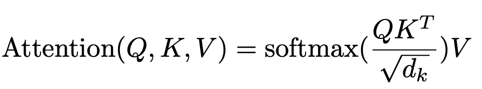
There's a lot going on here, but I'll break things down step by step.

Below is the above formula shown with the shape of the tensor inputs and outputs, where n is the number of tokens in the input sequence and d is the dimensionality of those tokens. For example, if we were dealing with a sequence of words the dimensionality d would be the dimension of the word embeddings for the n tokens in the sequence.

Note: here I ignore the softmax and sqrt(d_k) scaling term in the attention equation for visual simplicity, but I'll discuss those later.

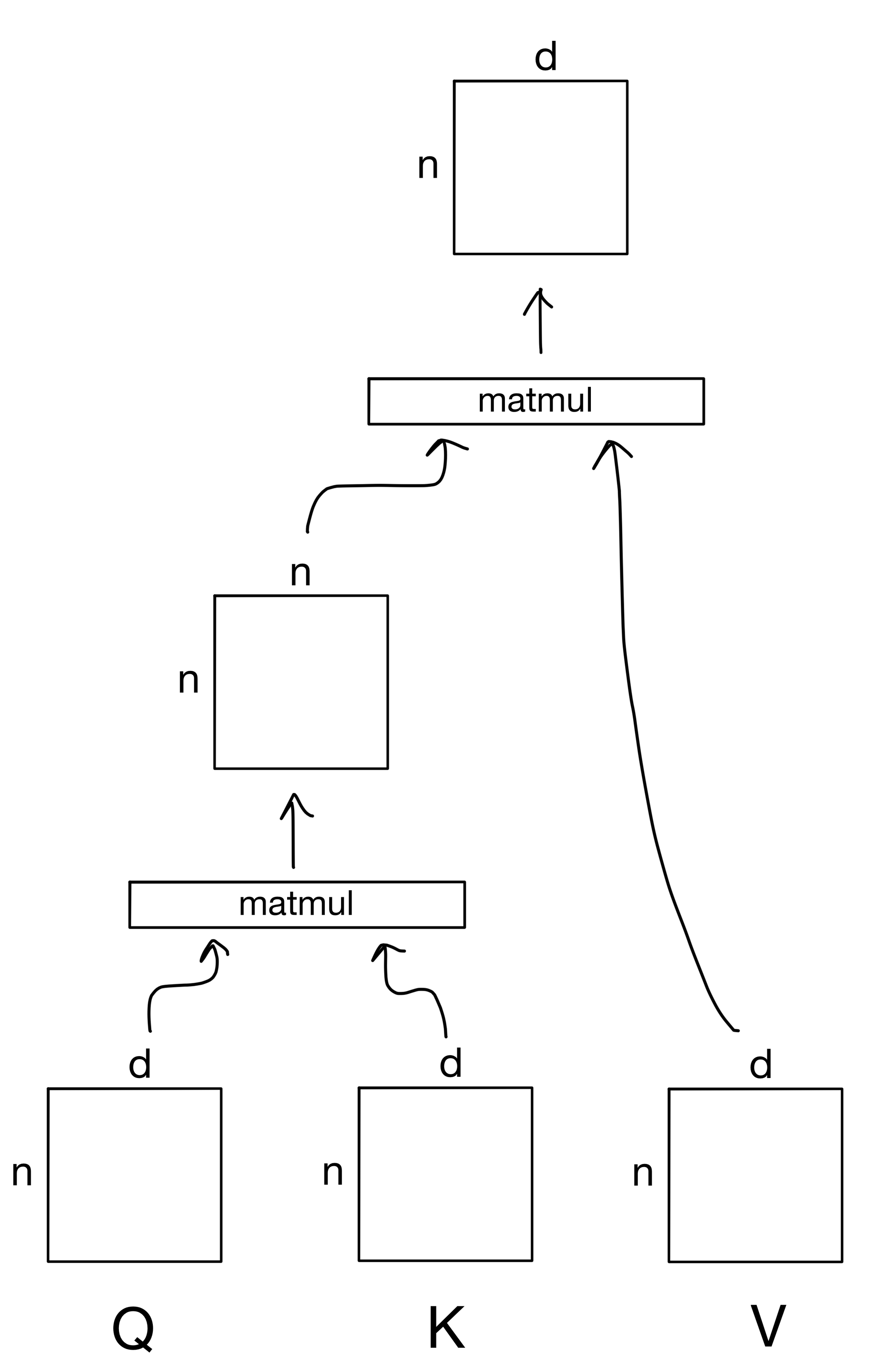
There are three main inputs to the attention mechanism: queries (Q), keys (K), and values (V). These inputs can all be described in terms of a "information retrieval" system of sorts. The general idea is that we submit a query for each token in the input sequence. We then take those queries and match them against a series of keys that describe values that we want to know something about. The similarity of a given query to the keys determines how much information from each value to retrieve for that particular query

For now, don't worry too much about where Q, K, and V come from, I'll talk about that more extensively in part 2 of the post. However, for now, they typically are are each a separate linear transformation of the same input matrix. So the attention operation is an effective way of spreading information between tokens of the same sequence. This is known as self attention. The same mechanism can also be used with tokens in a different sequence, but more on that next week.

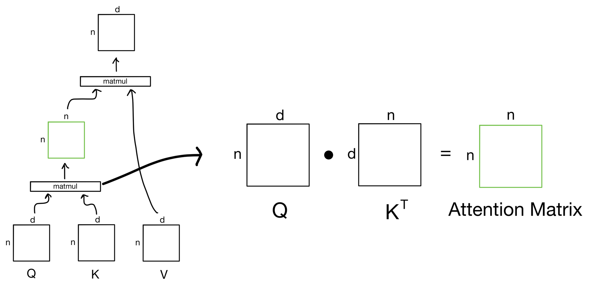
The Attention Matrix

The output of the first matrix multiplication, where we take the similarity of each query to each of the keys, is known as the attention matrix. The attention matrix depicts how much each token in the sequence is paying attention to each of the keys (hence the n x n shape). If we zoom in to our earlier depiction of the attention operation we see the matrix multiplication to produce the attention matrix.

But what's the intuition behind why this matrix multiplication between the queries and keys works?

Before answering the above, let's quickly review what the dot product between two vectors represents. For two vectors whose direction is similar the dot product will be large, while for two vectors pointing in different directions the dot product will be small.

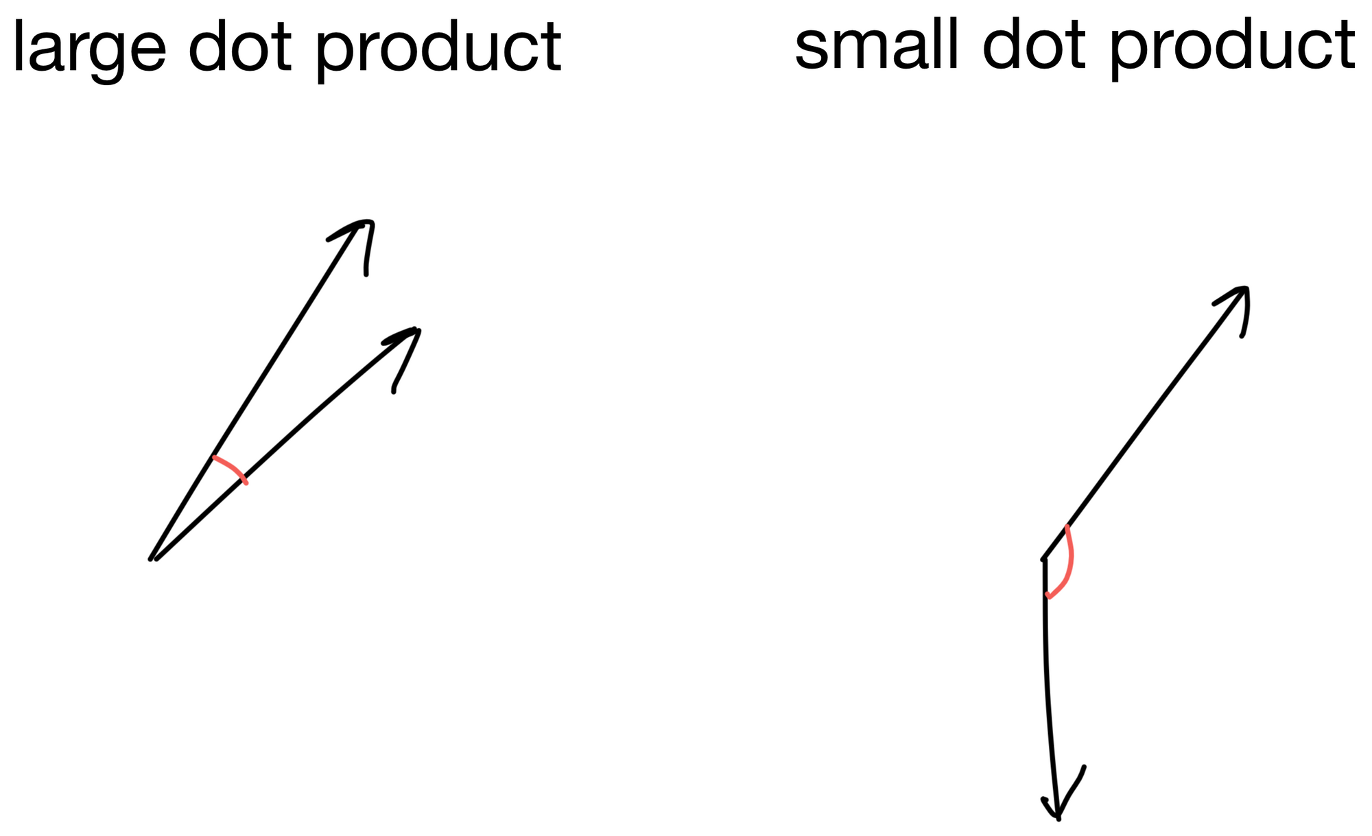
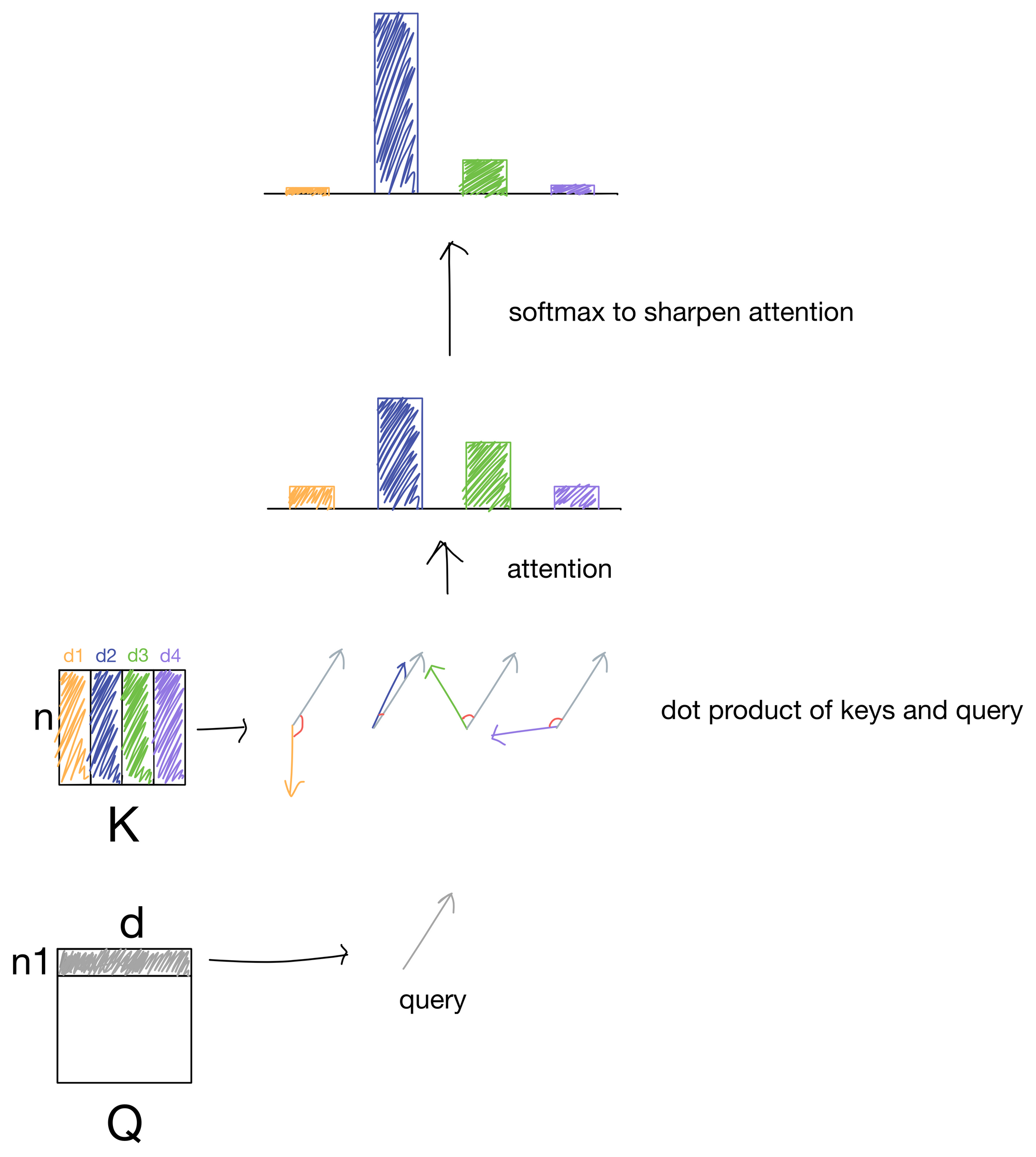
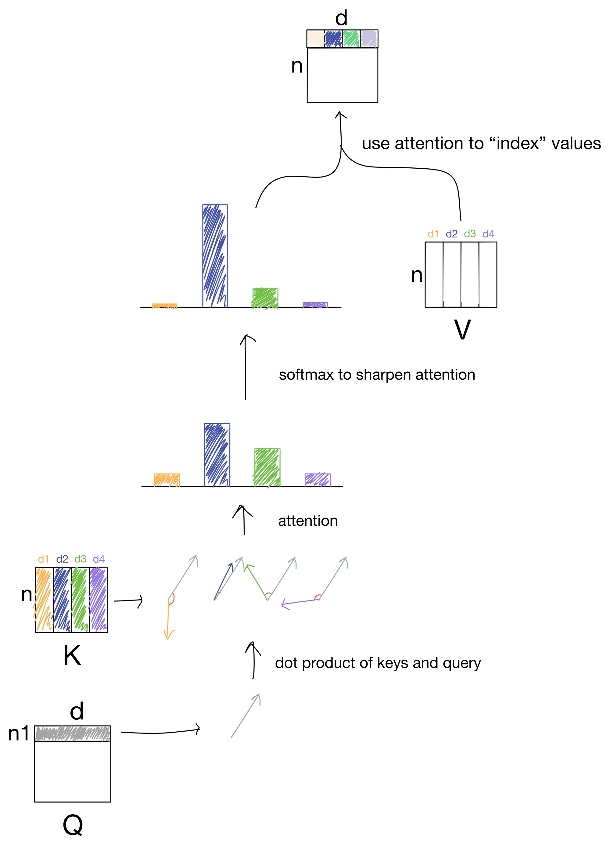
Let us now think of our queries as a series of vectors, one for each token in the input matrix. We take the dot product of each query vector with each key (of which there are four in this simple description, d1-4).

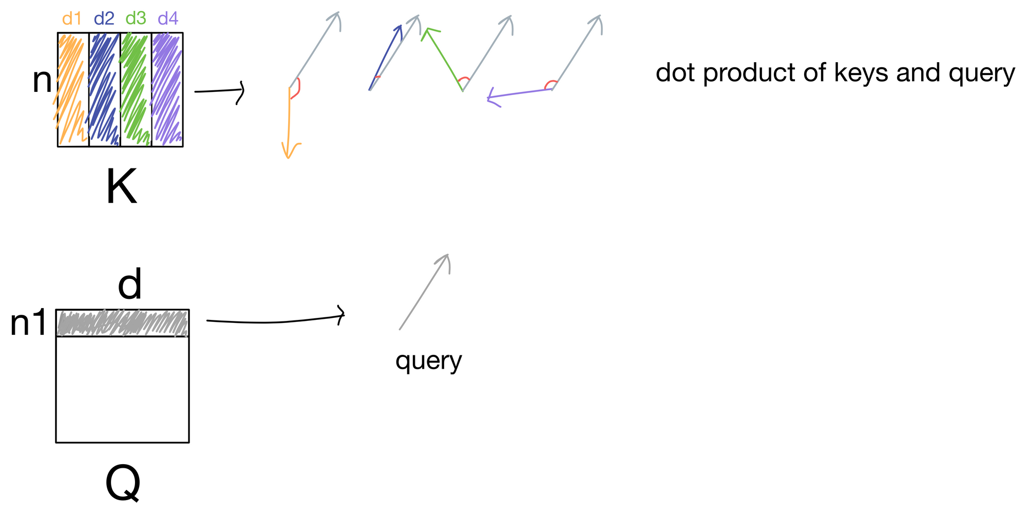
In the above illustration, we take the dot product for a single query with each key and are left with four scalar values. For keys close to the same direction as the query, the values will be large, while for keys differing in direction from the query vector the values would be low. These values are then passed through a softmax function to scale the values to a probability distribution that adds up to 1, and also sharpens the distribution so the higher values are even higher and lower values even lower. These values are what make up the attention matrix, and are a representation of how much each query matches a given key. Since typically the queries and keys are derived from the same sequence of input tokens, the attention values indicate how much each token in the sequence is "paying attention" to other tokens in the sequence.

Quick note: before the softmax function the attention values are typically scaled by the square root of the number of keys (i.e. tokens in the sequence), but I don't show it visually for simplicity.

Routing Information

After we have our attention values, we need to index the information contained in the value matrix V, because, after all, now that we know how we want to route information, we need to actually route the information contained in the values.

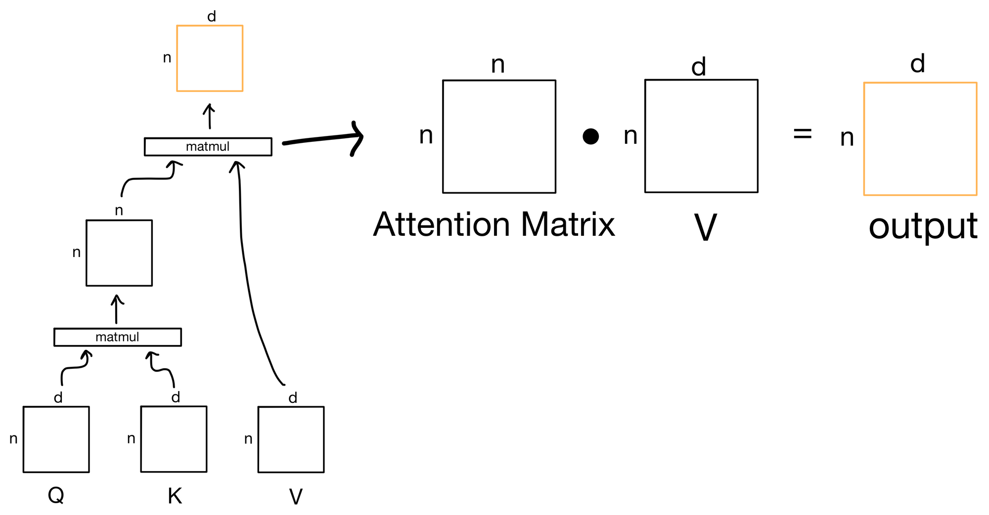
To route the information, we simply take another dot product, but this time between the attention matrix and the value matrix.

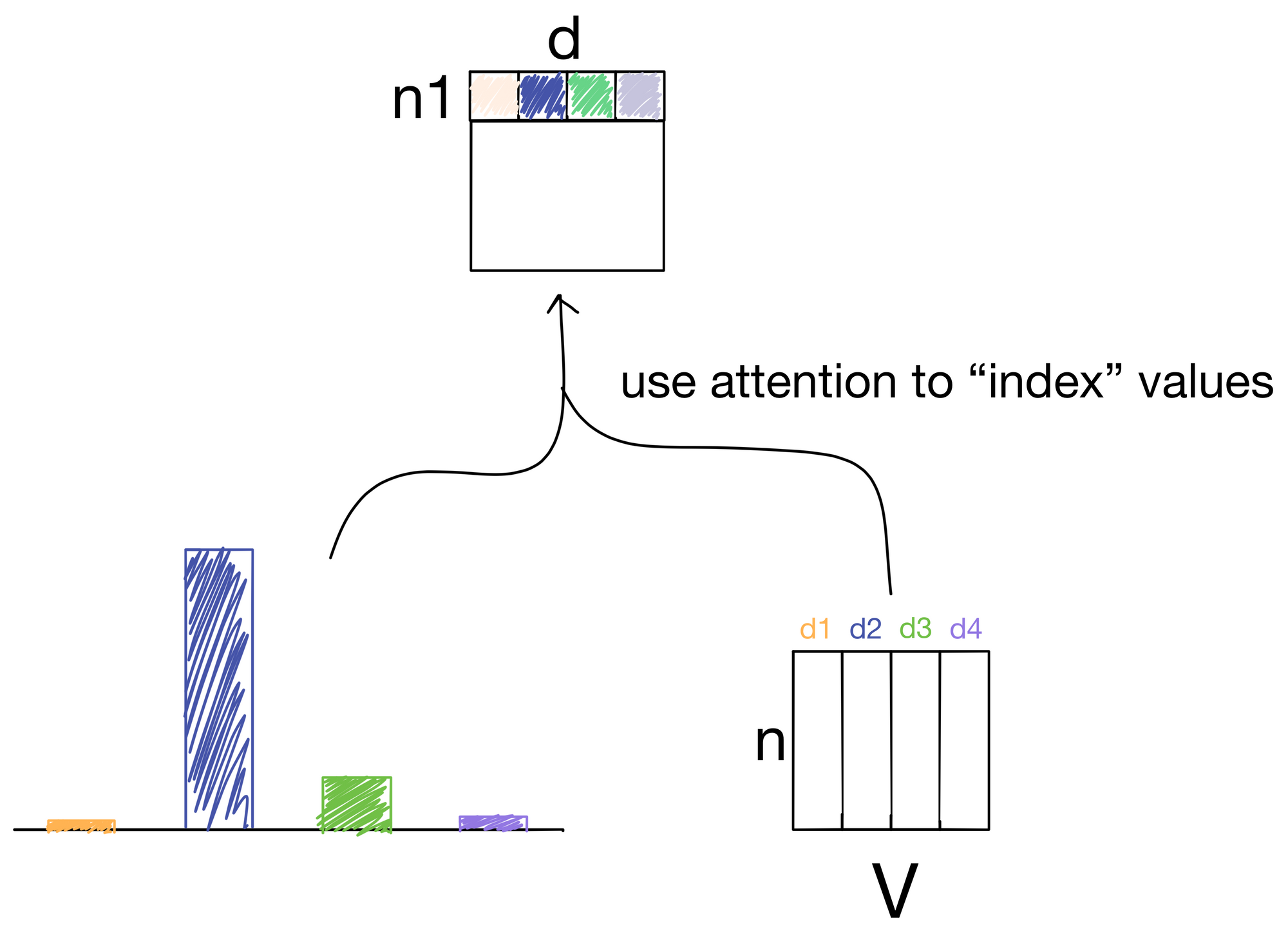
In doing so we effectively "index" into the information for each value in the value matrix in proportion with the amount attention described in the attention matrix.

At the end of all this we in theory have a better, more information rich representation than prior to the attention operation.

So there we have it, the attention mechanism.

There are a few additional twists, such as multi-head attention, which is used in transformers architectures. But we'll dive into that next week when we explore how the attention mechanism is used in neural network encoders and decoders.

Hope to see you then :)

1. ViT: https://arxiv.org/abs/2010.11929
2. Transformer: https://arxiv.org/abs/1706.03762
3. BERT: https://arxiv.org/abs/1810.04805v2